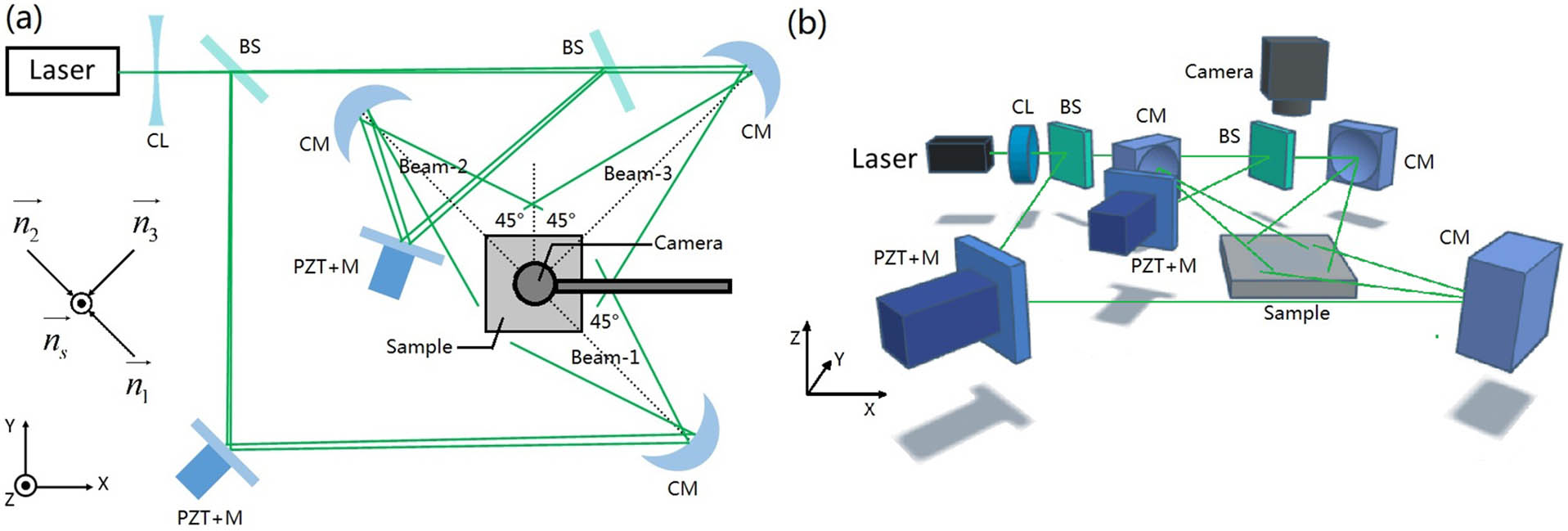
Fig. 1. Setup for ESPI measurement. (a) Top view; (b) 3D view. The camera is above the sample to take pictures of its surface. The height and focus of the camera can be adjusted to get different magnifications. Laser, CNI MSL-532 (diode-pumped solid-state laser, 532 nm, 20 mW). Camera, Flea^®3 FL3-U3-13S2M-CS 1/3” monochrome USB 3.0 Camera. CL, concave lens; CM, concave mirror; BS, beam splitter; $\mathrm{PZT}+\mathrm{M}$, piezo-actuated mirror.

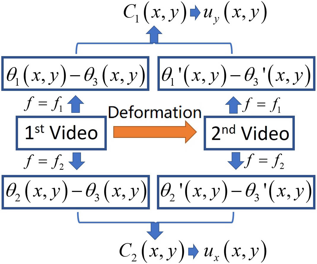
Fig. 2. Flowchart of the 2D displacement measurement.

Fig. 3. Term $\cos ({\theta }_1-{\theta }_2+a\sin 2\pi f_{1}t-a\sin 2\pi f_{2}t)$ represented in the frequency domain with $t=0\mathrm{s}$, $1/63\mathrm{s},2/63\mathrm{s},...,62/63\mathrm{s}$. $a$ is set to be 2.4048 rad, $f_1=9\mathrm{Hz}$, and $f_2=7\mathrm{Hz}$. Here, we have arbitrarily set ${\theta }_1=0.2\mathrm{rad}$, and ${\theta }_2=0.9\mathrm{rad}$.

Fig. 4. Bending specimen (photo taken by a camera that is not used in the experiments). By adjusting the micrometer screw, different deformation states can be obtained. The white rectangle represents the zone of interest.

Fig. 5. Phase images (without filtering) showing the displacement field along the $Y$ axis and $X$ axis obtained with sinusoidal phase modulations. A phase difference of $2\pi$ represents a displacement difference of about 385 nm. The micrometer screw advances 10 and 50 μm, respectively, along the $Y$ axis. The generalized lock-in detection^[9,11,12] is used to process data.

Fig. 6. From phase images to quantitative 2D strain field. (a), (b) Unfiltered phase images (we took the central parts of Figs. 5(c) and 5(d) as examples). (c), (d) Filtered phase images. (e), (f) Displacements $u_y$ and $u_x$. (g), (h) Normal strains ${\epsilon }_y$ and ${\epsilon }_x$. (i) Shear strain ${\gamma }_{xy}$.

Fig. 7. Phase images (without filtering) showing the displacement field along the $Y$ axis and $X$ axis obtained with linear/sawtooth phase modulations. A phase difference of $2\pi$ represents a displacement difference of about 385 nm. The micrometer screw advances 50 μm along the $Y$ axis. The lock-in detection^[9] is used to process data.