Simultaneous 2D in-plane deformation measurement using electronic speckle pattern interferometry with double phase modulations

Yunlong Zhu; Julien Vaillant; Guillaume Montay; Manuel François; Yassine Hadjar; Aurélien Bruyant

doi:10.3788/COL201816.071201

Abstract

Electronic speckle pattern interferometry (ESPI) and digital speckle pattern interferometry are well-established non-contact measurement methods. They have been widely used to carry out precise deformation mapping. However, the simultaneous two-dimensional (2D) or three-dimensional (3D) deformation measurements using ESPI with phase shifting usually involve complicated and slow equipment. In this Letter, we solve these issues by proposing a modified ESPI system based on double phase modulations with only one laser and one camera. In-plane normal and shear strains are obtained with good quality. This system can also be developed to measure 3D deformation, and it has the potential to carry out faster measurements with a high-speed camera.

In-plane deformations can be easily measured by a simple electronic speckle pattern interferometry (ESPI) measuring system^[1]. In such a system, the temporal phase-shifting technique is often applied for phase retrieval to improve the performance^[2]. However, in a standard two-beam configuration, only one displacement component is measured.

In order to measure the two-dimensional (2D) in-plane displacement field [or the whole three-dimensional (3D) displacement field], several solutions have been proposed. The most direct one is to use digital speckle photography (DSP) (or to combine DSP with out-of-plane ESPI for the 3D measurement)^[3]. Nevertheless, the sensitivity of DSP is not as good as that of ESPI. A natural solution is then to combine ESPI measuring systems^[4,5]. More recently, in-plane ESPI measurement systems were notably combined with out-of-plane ESPI to perform 3D analysis using optical switches, though with a limited time resolution (for example, the acquisition time for the “ $Q$ -300 3D-ESPI System” is 3.5 s for 3D analysis), due to the iterative process requirement^[6–8]. To solve the time issue, a spatial phase-shifting technique can be applied^[6]; however, it often makes the system substantially more complex and expensive.

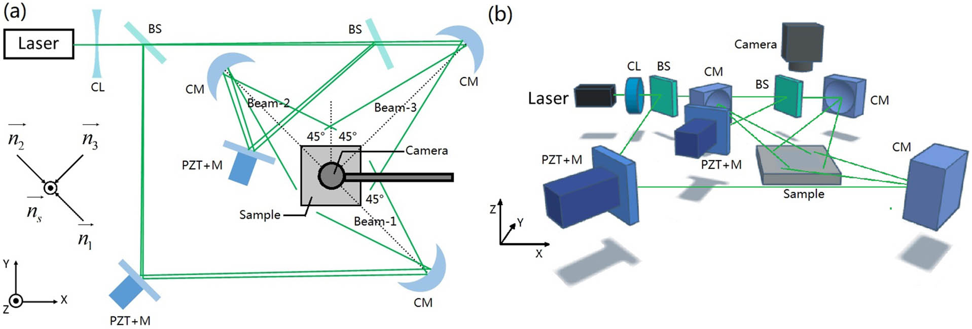
In this Letter, we show the possibility of doing simultaneous 2D measurement using the widely recognized ESPI technique and a single laser without switches. The optical arrangement is shown in Fig. 1. There are three coherent laser beams originating from a single laser: Beam 1, Beam 2, and Beam 3. The phases of Beam 1 and Beam 2 can be modulated by the corresponding piezo-actuated mirrors. When two temporal phase modulation functions, $F_{1} (t)$ and $F_{2} (t)$ , are applied to them, respectively, the scalar light field of the subjective speckles $E (x, y)$ can be expressed as $E (x, y) = A_{1} (x, y) e^{i [2 π f_{c} t + θ_{1} (x, y) + F_{1} (t)]} + A_{2} (x, y) e^{i [2 π f_{c} t + θ_{2} (x, y) + F_{2} (t)]} + A_{3} (x, y) e^{i [2 π f_{c} t + θ_{3} (x, y)]} .$ (1)

Sign up for Chinese Optics Letters TOC. Get the latest issue of Chinese Optics Letters delivered right to you！Sign up now

Figure 1.Setup for ESPI measurement. (a) Top view; (b) 3D view. The camera is above the sample to take pictures of its surface. The height and focus of the camera can be adjusted to get different magnifications. Laser, CNI MSL-532 (diode-pumped solid-state laser, 532 nm, 20 mW). Camera, Flea^®3 FL3-U3-13S2M-CS 1/3” monochrome USB 3.0 Camera. CL, concave lens; CM, concave mirror; BS, beam splitter; $PZT + M$ , piezo-actuated mirror.

$A_{m} (x, y)$ and $θ_{m} (x, y)$ are the amplitude and the initial phase of Beam $m$ ( $m = 1, 2, 3$ ) at point ( $x$ , $y$ ), respectively, and $f_{c}$ is the optical frequency of the laser.

On the sample surface, the light intensity $I (x, y)$ can be expressed as $I (x, y) \propto {| E (x, y) |}^{2} = [A_{1}^{2} (x, y) + A_{2}^{2} (x, y) + A_{3}^{2} (x, y)] + 2 A_{1} (x, y) A_{2} (x, y) \cos [θ_{1} (x, y) + F_{1} (t) - θ_{2} (x, y) - F_{2} (t)] + 2 A_{1} (x, y) A_{3} (x, y) \cos [θ_{1} (x, y) + F_{1} (t) - θ_{3} (x, y)] + 2 A_{2} (x, y) A_{3} (x, y) \cos [θ_{2} (x, y) + F_{2} (t) - θ_{3} (x, y)] .$ (2)

After a small displacement $u (x, y)$ , the light intensity turns into $I^{'} (x, y) \propto {| E^{'} (x, y) |}^{2} = [A_{1}^{2} (x, y) + A_{2}^{2} (x, y) + A_{3}^{2} (x, y)] + 2 A_{1} (x, y) A_{2} (x, y) \cos [θ_{1}^{'} (x, y) + F_{1} (t) - θ_{2}^{'} (x, y) - F_{2} (t)] + 2 A_{1} (x, y) A_{3} (x, y) \cos [θ_{1}^{'} (x, y) + F_{1} (t) - θ_{3}^{'} (x, y)] + 2 A_{2} (x, y) A_{3} (x, y) \cos [θ_{2}^{'} (x, y) + F_{2} (t) - θ_{3}^{'} (x, y)],$ (3)with $θ_{1}^{'} (x, y) = θ_{1} (x, y) + \frac{2 π}{λ} (n_{1} - n_{s}) \cdot u (x, y),$ (4) $θ_{2}^{'} (x, y) = θ_{2} (x, y) + \frac{2 π}{λ} (n_{2} - n_{s}) \cdot u (x, y),$ (5) $θ_{3}^{'} (x, y) = θ_{3} (x, y) + \frac{2 π}{λ} (n_{3} - n_{s}) \cdot u (x, y),$ (6)where $λ$ is the wavelength of the laser, $n_{m}$ is the unit vector along the illumination direction of Beam $m$ ( $m = 1, 2, 3$ ), and $n_{s}$ is the unit vector along the viewing direction. $n_{m}$ and $n_{s}$ can be roughly considered to be the same for every point ( $x$ , $y$ ) on the sample surface.

If we choose the following linear (or sawtooth) modulation functions: $F_{1} (t) = 2 π f_{1} t,$ (7) $F_{2} (t) = 2 π f_{2} t,$ (8)then we have $I (x, y) \propto {| E (x, y) |}^{2} = [A_{1}^{2} (x, y) + A_{2}^{2} (x, y) + A_{3}^{2} (x, y)] + 2 A_{1} (x, y) A_{2} (x, y) \cos [θ_{1} (x, y) - θ_{2} (x, y) + 2 π (f_{1} - f_{2}) t] + 2 A_{1} (x, y) A_{3} (x, y) \cos [θ_{1} (x, y) - θ_{3} (x, y) + 2 π f_{1} t] + 2 A_{2} (x, y) A_{3} (x, y) \cos [θ_{2} (x, y) - θ_{3} (x, y) + 2 π f_{2} t] .$ (9)

Obviously, when $f_{1}$ , $f_{2}$ and $| f_{1} - f_{2} |$ are not equal to each other with a lock-in detection at $f_{1}$ , $θ_{1} (x, y) - θ_{3} (x, y)$ can be extracted; with a lock-in detection at $f_{2}$ , $θ_{2} (x, y) - θ_{3} (x, y)$ can be extracted^[9]. The same procedure can be carried out to obtain $θ_{1}^{'} (x, y) - θ_{3}^{'} (x, y)$ and $θ_{2}^{'} (x, y) - θ_{3}^{'} (x, y)$ . If we set $C_{1} (x, y) = [θ_{1}^{'} (x, y) - θ_{3}^{'} (x, y)] - [θ_{1} (x, y) - θ_{3} (x, y)],$ (10) $C_{2} (x, y) = [θ_{2}^{'} (x, y) - θ_{3}^{'} (x, y)] - [θ_{2} (x, y) - θ_{3} (x, y)],$ (11)then, according to Eq. (4)–(6), we have $C_{1} (x, y) = \frac{2 π}{λ} (n_{1} - n_{3}) \cdot u (x, y),$ (12) $C_{2} (x, y) = \frac{2 π}{λ} (n_{2} - n_{3}) \cdot u (x, y) .$ (13)

The $z$ components of $n_{1}$ , $n_{2}$ , and $n_{3}$ are almost equal, so they will cancel each other out in Eqs. (12) and (13). Concerning the $x$ and $y$ components of $n_{1}$ , $n_{2}$ , and $n_{3}$ , we can see from Fig. 1 that $(n_{1} - n_{3})$ is parallel to the $Y$ axis, and $(n_{2} - n_{3})$ is parallel to the $X$ axis. So, $C_{1} (x, y)$ and $C_{2} (x, y)$ can be expressed as $C_{1} (x, y) = g \cdot u_{y} (x, y),$ (14) $C_{2} (x, y) = g \cdot u_{x} (x, y),$ (15)where $g$ is a measurable constant, $u_{x} (x, y)$ and $u_{y} (x, y)$ are the $x$ and $y$ components of $u (x, y)$ , respectively. This means the 2D in-plane displacement field can be measured. The whole procedure is briefly illustrated in Fig. 2.

Figure 2.Flowchart of the 2D displacement measurement.

This method can also be extended to carry out 3D displacement field measurements without increasing acquisition time and without an additional laser or camera: if the laser is separated into a fourth coherent beam and its direction of illumination is $n_{4}$ , then this system can be used to measure the 3D displacement field, as long as $n_{4} - n_{3}$ has a non-zero $z$ component, and this fourth beam is modulated at an appropriate frequency.

It should be noticed that when piezoelectric actuators are driven to make sawtooth displacements, the precision cannot be guaranteed, especially at a high frequency, where the fly-back time of the mirror cannot be neglected. The nonlinearity and noise generated by the sudden return becomes unacceptable when high-speed measurement is required. This issue can be addressed with sinusoidal phase modulations such as $F_{1} (t) = a \sin 2 π f_{1} t,$ (16) $F_{2} (t) = a \sin 2 π f_{2} t,$ (17)where $a$ is the amplitude of phase modulation. It should be noticed that $f_{1}$ and $f_{2}$ are not randomly chosen. It is favorable to choose coprime integers, as will be detailed later. Now we have $I (x, y) \propto {| E (x, y) |}^{2} = [A_{1}^{2} (x, y) + A_{2}^{2} (x, y) + A_{3}^{2} (x, y)] + 2 A_{1} (x, y) A_{2} (x, y) \cos [\begin{matrix} θ_{1} (x, y) - θ_{2} (x, y) \end{matrix} \begin{matrix} + a \sin 2 π f_{1} t - a \sin 2 π f_{2} t] \end{matrix} + 2 A_{1} (x, y) A_{3} (x, y) \cos [θ_{1} (x, y) - θ_{3} (x, y) + a \sin 2 π f_{1} t] + 2 A_{2} (x, y) A_{3} (x, y) \cos [θ_{2} (x, y) - θ_{3} (x, y) + a \sin 2 π f_{2} t] .$ (18)

In Eq. (18), according to the Jacobi–Anger expansion, in the frequency domain, the third term will be distributed at the integer multiples of $f_{1}$ , and the fourth term will be distributed at the integer multiples of $f_{2}$ . If we set $a = 2.4048 rad$ , so that $J_{0} (a) = 0$ ( $J_{0}$ is the zeroth Bessel function of the first kind), then both of them will not contain any signal at 0 Hz. So, in the frequency domain, they will not overlap with each other until the least common multiple of $f_{1}$ and $f_{2}$ , which is 63 Hz in our case ( $f_{1} = 9 Hz$ , $f_{2} = 7 Hz$ , 9 and 7 are coprime integers). This means these two terms can be efficiently separated.

As for the second term in Eq. (18), we can make use of the trigonometric formulas (sum/difference identities) to get $\cos [θ_{1} (x, y) - θ_{2} (x, y) + a \sin 2 π f_{1} t - a \sin 2 π f_{2} t] = \cos [θ_{1} (x, y) - θ_{2} (x, y)] \cos (a \sin 2 π f_{1} t) \cos (a \sin 2 π f_{2} t) - \cos [θ_{1} (x, y) - θ_{2} (x, y)] \sin (a \sin 2 π f_{1} t) \sin (a \sin 2 π f_{2} t) - \sin [θ_{1} (x, y) - θ_{2} (x, y)] \sin (a \sin 2 π f_{1} t) \cos (a \sin 2 π f_{2} t) + \sin [θ_{1} (x, y) - θ_{2} (x, y)] \cos (a \sin 2 π f_{1} t) \sin (a \sin 2 π f_{2} t) .$ (19)

If we analyze the first term in Eq. (19) with the Jacobi–Anger expansion when $J_{0} (a) = 0$ , then we have $\cos (a \sin 2 π f_{1} t) \cos (a \sin 2 π f_{2} t) = 4 \sum_{p = 1}^{\infty} \sum_{q = 1}^{\infty} J_{2 p} (a) J_{2 q} (a) \cos (2 p \cdot 2 π f_{1} t) \cos (2 q \cdot 2 π f_{2} t),$ (20)with $\cos (2 p \cdot 2 π f_{1} t) \cos (2 q \cdot 2 π f_{2} t) = \frac{1}{2} \cos (2 p \cdot 2 π f_{1} t + 2 q \cdot 2 π f_{2} t) + \frac{1}{2} \cos (2 p \cdot 2 π f_{1} t - 2 q \cdot 2 π f_{2} t),$ (21)where $p$ and $q$ are positive integers. Through Eq. (21), we know that this term contains signals at the frequencies of ( $| 2 p f_{1} \pm 2 q f_{2} |$ ). Likewise, by analyzing the other three terms in Eq. (19), it can be concluded that the second term in Eq. (18) contains ( $| p f_{1} \pm q f_{2} |$ ) signals.

Since $p$ and $q$ are positive integers, the solutions for $| p f_{1} \pm q f_{2} | = n f_{1}$ or $| p f_{1} \pm q f_{2} | = {n f}_{2}$ (n is a positive integer) can only be found when $p$ or $q$ is relatively large, which represents the high-frequency signal where the intensity is usually very small [since $J_{p} (a) \approx 0$ or $J_{q} (a) \approx 0$ ]. So, we can estimate that it will not have too much influence on the interesting frequencies. A simple simulation is done with $f_{1} = 9 Hz$ , and $f_{2} = 7 Hz$ , and the result is shown in Fig. 3 to illustrate this point.

Figure 3.Term $\cos (θ_{1} - θ_{2} + a \sin 2 π f_{1} t - a \sin 2 π f_{2} t)$ represented in the frequency domain with $t = 0 s$ , $1 / 63 s, 2 / 63 s, . . ., 62 / 63 s$ . $a$ is set to be 2.4048 rad, $f_{1} = 9 Hz$ , and $f_{2} = 7 Hz$ . Here, we have arbitrarily set $θ_{1} = 0.2 rad$ , and $θ_{2} = 0.9 rad$ .

We can now draw a direct link between the four terms in Eq. (18) and the frequency spectrum. The first term corresponds to the signal at 0 Hz, the third term corresponds to signals at $p f_{1}$ , the fourth term corresponds to signals at $q f_{2}$ , and the second term corresponds to signals at other frequencies. So, just like using linear modulation, information can be easily sorted out so that the 2D displacement field can be measured. In fact, by simply replacing the lock-in detection algorithm with the traditional sinusoidal phase modulation algorithm (see Ref. [10]) or the recently proposed generalized lock-in detection algorithm (see Refs. [9,11,12]), the needed phase information can be obtained. Likewise, while dealing with the same set of data, if we set the demodulation frequency at $f_{1}$ in the algorithm, then we can get $C_{1} (x, y)$ ; if we set it at $f_{2}$ , then we can get $C_{2} (x, y)$ . With $C_{1} (x, y)$ and $C_{2} (x, y)$ , the 2D displacement field $u_{x} (x, y)$ and $u_{y} (x, y)$ can be obtained.

We used a bending specimen, as shown in Fig. 4. It is a test sample fabricated by the company HOLO 3^[13].

Figure 4.Bending specimen (photo taken by a camera that is not used in the experiments). By adjusting the micrometer screw, different deformation states can be obtained. The white rectangle represents the zone of interest.

First, we make sure that there is already an initial contact between the micrometer screw and the bending specimen. Then, the two phase modulations are turned on, and a short video (1 s, 63 frames per second) is recorded. Likewise, we record another video after turning the micrometer screw so that the deformation state changes. By analyzing these two videos, we can measure the 2D displacement field.

When applying sinusoidal phase modulations described by Eqs. (16) and (17) with $f_{1} = 9 Hz$ , and $f_{2} = 7 Hz$ , we successfully obtained phase images ( $C_{1}$ and $C_{2}$ ), as shown in Fig. 5. The fringe visibility is very good; besides, very fine fringes can be observed on the left part of Figs. 5(a) and 5(b).

Figure 5.Phase images (without filtering) showing the displacement field along the $Y$ axis and $X$ axis obtained with sinusoidal phase modulations. A phase difference of $2 π$ represents a displacement difference of about 385 nm. The micrometer screw advances 10 and 50 μm, respectively, along the $Y$ axis. The generalized lock-in detection^[9,11,12] is used to process data.

From the obtained phase images (Fig. 5), we can quantitatively measure the 2D deformation (Fig. 6). First, the original phase images [Figs. 6(a) and 6(b)] were filtered with the conventional 2D convolution method [see Figs. 6(c) and 6(d)]. Then, they are 2D unwrapped to get smooth phase images, and the displacements $u_{y}$ and $u_{x}$ [Figs. 6(e) and 6(f)] can be calculated by Eqs. (14) and (15). The strains $ε_{y}$ , $ε_{x}$ , and $γ_{x y}$ can be quantitatively measured [Figs. 6(g), 6(h), 6(i)] for any choice of origins for $u_{y}$ and $u_{x}$ .

Figure 6.From phase images to quantitative 2D strain field. (a), (b) Unfiltered phase images (we took the central parts of Figs. 5(c) and 5(d) as examples). (c), (d) Filtered phase images. (e), (f) Displacements $u_{y}$ and $u_{x}$ . (g), (h) Normal strains $ε_{y}$ and $ε_{x}$ . (i) Shear strain $γ_{x y}$ .

When applying linear/sawtooth phase modulations described by Eqs. (7) and (8), similar fringes (see Fig. 7) are obtained, since the modulation frequencies are quite low ( $f_{1} = 9 Hz$ , and $f_{2} = 7 Hz$ ). However, the sawtooth approach will become much less efficient at higher speeds. There are some small differences in the fringe pattern, which are mainly due to phase noise, initial phase adjustment, and the fact that the loading processes were done manually and are not perfectly reproducible.

Figure 7.Phase images (without filtering) showing the displacement field along the $Y$ axis and $X$ axis obtained with linear/sawtooth phase modulations. A phase difference of $2 π$ represents a displacement difference of about 385 nm. The micrometer screw advances 50 μm along the $Y$ axis. The lock-in detection^[9] is used to process data.

Compared to previous reports of 2D in-plane displacement field measurements, the proposed approach is much simpler with only one laser and one camera; yet, high-quality fringes have been obtained. A camera with moderate speed (63 frames per second) is used; still, the data acquisition time (1 s for 2D information) is even a little advantageous over some commercialized systems (e.g. 3.5 s for 3D information^[8]). Obviously, this system has the potential to be operated at a high speed while providing accurate results by using the sinusoidal phase modulation together with a high-speed camera. Although the relatively voluminous data may be a challenge for lower-end computers to carry out real-time analysis, it does not seem to be a problem for the future, since the semiconductor industry is developing rapidly. Last but not least, this approach has the potential to carry out simultaneous ESPI measurements of the 3D displacement field.

References

[1] R. Jones, C. Wykes. Holographic and Speckle Interferometry(1989).

[2] K. Creath. Appl. Opt., 24, 3053(1985).

[3] J. Li, S. Li, Y. Sun, H. An. Proc. SPIE, 4183, 309(2001).

[4] A. J. Moore, J. R. Tyrer. Meas. Sci. Technol., 1, 1024(1990).

[5] L. Yang, X. Xie, L. Zhu, S. Wu, Y. Wang. Chin. J. Mech. Eng., 27, 1(2014).

[6] X. Xie, L. Yang, X. Chen, N. Xu, Y. Wang. Proc. SPIE, 8916, 89160D(2013).

[7] L. Yang, A. Ettemeyer. Opt. Eng., 42, 1257(2003).

[8] 3D ESPI System (Q-300).

[9] Y. Zhu, J. Vaillant, M. François, G. Montay, A. Bruyant. Appl. Opt., 56, F97(2017).

[10] O. Sasaki, H. Okazaki. Appl. Opt., 25, 3137(1986).

[11] A. Bruyant, J. Vaillant, T. H. Wu, Y. Zhu, Y. Huang, A. Al Mohtar. Interferometry using generalized lock-in amplifier (G-LIA): a versatile approach for phase-sensitive sensing and imaging. Optical Interferometry(2017).

[12] A. Al Mohtar, J. Vaillant, Z. Sedaghat, M. Kazan, L. Joly, C. Stoeffler, J. Cousin, A. Khoury, A. Bruyant. Opt. Express, 22, 22232(2014).

[13] Products and technologies–deformations.