Discovering the physics and dynamics of the solid earth is essential to meet the challenges of natural hazards, energy crisis, and climate changes. Solid earth geoscience is a data-driven filed which demands large datasets of geological events¹. For geoscience data acquisition, it is required to sense the earth’s crustal deformation with a strain resolution less than 10^-9 ε in a frequency region from static to 100 Hz². Moreover, in order to refine the structure image of the errors induced by the Earth crustal damage, the strain sensing for geoscience research requires denser spatial coverage of individual sensors and more accurate recording instruments³. The broadband seismometer networks represent the state of arts technology and provide high quality Earth crustal deformation waveforms with broadband frequency content⁴. However, the dense seismometer networks deployed in areas where access and power supply are limited will consume a great effort and resources⁵.

Recently, optical fiber strain sensor has attracted considerable research interests for geoscience applications, owing to their unique advantages of passive, multiplexing, and anti-electromagnetic interference⁶. For instance, optical fiber Bragg grating (FBG) based sensors have been widely exploited to monitor the earth tide, which possess a minimum static strain resolution of 270 pε². However, the multiplexing capacity of the FBG strain sensors is limited by the bandwidth of the reflection spectrum. Moreover, the signal crosstalk between the sensors in the FBG sensor network will increase the noise floor of measurement⁷. Hence, the sensing range and spatial coverage density of the high-quality single point optical fiber sensor networks should be further promoted.

As an alternative approach, optical fiber distributed acoustic sensor (DAS), which offers a long sensing distance without blind area^{8, 9}, has demonstrated efficient seismic acquisition ability in seismology application such as natural hazard prediction and crust exploration^{10, 11}. In general, DAS, which is realized based on phase-sensitive optical time domain reflectometry (φ-OTDR) technology, can interrogate the strain and temperature variations along the entire length of an optical fiber^{12, 13}. With current technologies, DAS has achieved a dynamic strain resolution down to nano-strain level¹⁴. Moreover, the quasi-DAS assisted with ultra-weak FBG array has been proposed with pico-strain dynamic resolution above 10 Hz frequency range^{15, 16}. Due to the high sensitivity, high spatial and temporal resolution, DAS has been developed and used for broadband seismic monitoring in oil/gas exploration¹⁷. Nevertheless, the frequency shift of the laser source, as well as the cross-sensitivity between temperature and strain, severely ruin the signal to noise ratio (SNR) of the DAS in low frequency band^{18, 19}. The noise in ultra-low frequency band of the DAS system limits the availabilities for nature earthquake recording and earth tide monitoring. In order to improve the sensing performance in low-frequency domain, many efforts have been done to suppress the phase drift of the φ-OTDR. F. Zhu proposed an active compensation method to reduce the laser frequency shift influence by tracking and comparing the OTDR intensity traces with different frequencies¹⁹. But the response time of this method will be limited by the number of tuning frequencies. Furthermore, Q. Yuan has demonstrated the twice differential method to compensate the influence of laser frequency shift, and successfully detected the strain variation with amplitude of 5.9 nε at 0.1 Hz²⁰. However, the strain resolution of the DAS in the mHz range is still much worse than the high-quality single point optical fiber sensor. Actually, the quasi-static measurement from mHz to Hz is essential to the solid earth geoscience research. To sense the mHz strain information with high sensitivity and dense spatial coverage, it is necessary for the ultra-low frequency noise of the DAS to be greatly suppressed.

In this paper, we demonstrated a high-resolution strain sensor network with large sensing capacity based on φ-OTDR technology and scatter enhanced points (SEPs) array. In the prototype system, the optical fiber with SEPs array is divided into sensing fiber and reference fiber. The reference fiber packaged with strain isolation is used to compensate the ultra-low frequency noise induced by laser source frequency shift and environmental temperature change. The characteristics of the above phase noise are systematically analyzed. Then, a hysteresis model based on the hysteresis operator and LS-SVM is introduced to reduce the thermal hysteresis between the sensing fiber and reference fiber. Assisted with the LS-SVM based hysteresis compensation scheme, a strain sensor network with high resolution in the ultra-low frequency and large sensing capacity is successfully achieved.

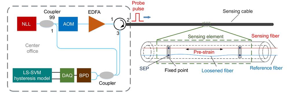
In order to achieve a large sensing capacity, the proposed high-resolution strain sensing network is interrogated by the φ-OTDR technology. The schematic diagram of the proposed sensing network for geoscience research is illustrated in Fig. 1. The sensing network consists of an interrogation office center and a special packaged sensing cable. In the interrogation system, an ultra-narrow linewidth laser (NKT x15) with linewidth of 100 Hz is used as a light source which is divided into a local oscillator laser and a probe laser by a 99:1 optical coupler. The probe laser is modulated into a series of pulses with frequency shift of 200 MHz by the acoustical optical modulator (AOM). After amplified by erbium doped fiber amplifier (EDFA), the pulses are injected into the sensing cable by a circulator. The backscattered light from the sensing cable is mixed with the local oscillator laser by a 50:50 coupler and then received by a balanced photodetector (BPD). Data acquisition card (DAQ) is used to acquire the heterodyne beat signals from the BPD.

The sensing cable is based on the specific packaged optical fiber with SEPs array²¹. The SEPs are inscribed by laser exposure on the single mode fiber (SMF) with a given interval. The scattering efficiency of the SEPs is improved by 10 dB compared to the Rayleigh scattering of the SMF²². A pair of SEPs along with the fiber between them compose one sensing section. The fiber with SEPs array is divided in to sensing fiber and reference fiber with the same SEPs number²³. The sensing fiber is for the sensing of strain, and the reference fiber is for the compensation of the phase drift induced by the environmental temperature and laser frequency variation. The sensing sections in the sensing fiber and reference fiber are respectively defined as sensing channels and reference channels. The SEPs of the sensing channels and the corresponding reference channels are aligned, and fixed with the sensing cable by epoxy curing agents. The sensing fiber in the cable is applied with a pre-strain for sensing of the strain of the cable. While the reference fiber is loosened in the cable to isolate the strain of the cable. Generally, the different packaging method will induce the length difference between the sensing fiber part and reference fiber part, which will introduce the different sensitivity for temperature and laser frequency vibration as well. However, the sensitivity difference between the sensing fiber part and reference fiber part is linear, which can be eliminated by linear fitting. When the spatial width of the injected probe pulse is shorter than the interval between two SEPs of the sensing section, the detected interference signal behaves as a series of beat frequency pulse trains, which can be described as:

$ I(t) = A\sum\limits_{n = 0}^N {[{\rm{rect}}\left(\frac{{t - {z_n} \cdot {n_0}/c}}{{{\tau _{\rm{p}}}}}\right) \cdot \cos (2{\rm{\pi}} {f_{\rm{d}}}t + }{\phi _n})]\;, $ (1)

where A is the amplitude of the interference signal, N is the number of the SEPs in the fiber, n₀ is the refractive index of the fiber core, c is the light speed in the vacuum, τ_p is the pulse width of the probe laser, z_n is the location of the n-th SEPs in the fiber, and φ_n is the phase of the scattering light of the n-th SEP. φ_n can be demodulated from the interference signal by the digital orthogonal phase discrimination method, which is deduced as:

${\phi _n} = {\rm{arctan}} (\frac{{{I_n}(t) \cdot \cos (2\pi {f_{\rm{d}}}t)}}{{{I_n}(t) \cdot \sin (2\pi {f_{\rm{d}}}t)}})\;,$ (2)

where I_n(t) is the interference signal scattering from the n-th SEP. Theoretically, the phase difference between two SEPs is only dependent on the change of optical path in the sensing section²⁴, which can be obtained by subtracting the phase of two SPEs in the sensing section, as expressed blow:

$\phi (k) = {\phi _{k + 1}} - {\phi _k} = \frac{{4 \rm{π} {n_0}\nu L{ε _k}}}{c}\;,$ (3)

where k=1,2, ···, N−1 is the number of the sensing section in the fiber, ν is the optical frequency of the laser, and ε_k is the strain applied on the k-th sensing section. When ν and n₀ are constant, the phase signal in the k-th sensing section will be only proportional to ε_k. However, it can be observed clearly that the phase signal of the sensing section φ(k) will be also influenced by variation of the laser frequency ν and refractive index n₀. Generally, the laser frequency ν will shift along with the environmental temperature drift, and the refractive index n₀ is also significantly influenced by the temperature variation of the fiber core. Thus, the laser frequency shift and fiber temperature fluctuation are the dominant noise sources in the ultra-low frequency domain.

In the proposed strain sensor network, a reference fiber with strain isolated package is employed to compensate the phase noise in low frequency band induced by environmental temperature and laser frequency shift. The compensation efficiency is dependent on the phase relationship between the sensing channel and corresponding reference channel. In order to investigate the phase variation characteristics, the laser frequency variation and temperature change were applied on the sensing cable for test. When the laser frequency variation with amplitude of 600 MHz and frequency of 1 Hz was introduced by frequency demodulation, the phase change of the sensing part and reference part are respectively plotted in the Fig. 2(a). The phase waveforms of the sensing channel and reference channel are identical with the variation of the laser frequency. Moreover, the relationship of the phase change between the sensing channel and reference channel is linear, which is illustrated in Fig. 2(b). Therefore, the phase noise induced by laser frequency shift can be compensated by direct differentiation.

Furthermore, the temperature fluctuation and the corresponding phase change are plotted in the Fig. 3(a), where the trigonometric temperature fluctuation with the amplitude of 5 °C was applied by a TEC. From Figs. 3(b) and 3(c), the hysteresis phenomenon can be observed between the temperature and phase. Moreover, the relationship between the phase change of the sensing channel and reference channel also exhibits an obvious hysteresis characteristic, as shown in the Fig. 3(d). The hysteresis stems from different temperature features induced by the different package methods, which will bring about a significant compensation error by direct differentiation. Therefore, a precision hysteresis model between the sensing channel and reference channel should be built to reduce the temperature compensation error.

Research on the hysteresis has a long history about a century. The Preisach model, which has been widely used for the modeling of hysteresis, has been developed based on incorporates relay operators^{25, 26}. Relay operator is the simplest example for a hysteresis nonlinearity, which is characterized by threshold a₁<a₂ and output values +1 and –1, as depicted in Fig. 4(a). For a given input x(t), the output of the Preisach model y(t) can be expressed as²⁷:

$ y(t) = \int_0^{ + \infty } {\int_{ - \infty }^{ + \infty } {d(r,s){R_{s - r,s + r}}[x](t)\rm{d}s\rm{d}r} }\;, $ (4)

where d(r, s) is the density function, R_s−r,s+r[∙] is the relay operator, r=(a₂−a₁)/2 is the half-width value, and s=(a₁+a₂)/2 is the mean value of the relay operator. A dividing curve, ψ(r, t), is defined to divide the relay operator into two distinct regions. The output value of the relay operator is +1 in the region below the curve and -1 in the region above the curve, respectively. The dividing curve ψ(r, t) can be considered as the play between two mechanical elements of relay. Therefore, a play operator P_r[x] is determined, and the corresponding input-output behavior is illustrated in Fig. 4(b). Mathematically, the play operator can be obtained by linear superposition of relay elements as follows²⁷:

$ \psi (r,t) = {P_r}[x](t) = \frac{1}{2}\int_{ - \infty }^{ + \infty } {{R_{s - r,s + r}}[x](t)\rm{d}s}\;. $ (5)

Therefore, the Preisach operator can be expressed as:

$ y(t) = \int_0^\infty {q(r,{P_r}[x](t))\rm{d}r} \;, $ (6)

where

$ q(r,s) = 2\int_0^s {w(r,\sigma )\rm{d}\sigma } \;. $ (7)

According to the general form in Eq. (7), the Preisach model can be decomposed into a continuous set of play operators and a one-to-one mapping function. Generally, the input-output relationship of the Preisach model can be defined as:

$ y(t) = F({P_r}[x](t))\;, $ (8)

where F(∙) is a function that maps the play operators set in the real-valued output y(t). Thus, the Preisach model can be implemented by approximating the mapping function based on the input and output value of real hysteresis materials through some identification methods, such as nonnegative least squares.

Least square support vector machine (LS-SVM) has been successfully introduced in modeling application for the global optimization property²⁸. Compared to the standard SVM, LS-SVM uses the least squared loss function instead of the ε-insensitive loss function. Hence, the analytical solutions of LS-SVM can be obtained by solving linear equations instead of quadratic programming problem. For a given training data set {(u_i, y_i), u_i∈Rⁿ, y_i∈R}, the LS-SVM model is expressed as:

$ y(u) = {{{w}}^{\rm{T}}} \cdot f(u) + b\;, $ (9)

where f(u) is the nonlinear mapping from the input space to higher feature space, w is the weight vector, and b is the bias. The optimization problem in the LS-SVM is obtained through the equation:

$ \begin{gathered} \min R({{w}},\xi ) = \frac{1}{2}{\left\| {{w}} \right\|^2} + C\sum\limits_i^n {\xi _i^2} \\ {\rm{s}}.{\rm{t}}.\;y_i = {{{w}}^{\rm{T}}} \cdot f({u_i}) + b + {\xi _i},i = 1,2,...,n\;, \\ \end{gathered} $ (10)

where C is the regularization parameters, and ξ_i is the error between the actual output and predictive output. The problem can be solved by defining the Lagrangian equation as follow:

$ L({{w}},b,\xi ,a) = R({{w}},\xi ) - \sum\limits_i^n {{a_i}({{{w}}^{\rm{T}}} \cdot f({u_i}) + b + {\xi _i} - {y_i})} \;, $ (11)

where a_i is the Lagrangian multiplier. The conditions for optimality are the saddle point of L, which can be found by solving the partial derivatives. After eliminating the w and ξ_i, the solution is given by the following linear equations:

$ \left[ {\begin{array}{*{20}{c}} 0&{{{{e}}^{\rm{T}}}} \\ {{e}}&{{{Ω}} + {{I}}/2C} \end{array}} \right]\left[ {\begin{array}{*{20}{c}} b \\ {{a}} \end{array}} \right] = \left[ {\begin{array}{*{20}{c}} 0 \\ {{y}} \end{array}} \right]\;, $ (12)

where e=[1, ···, 1]^T, y=[y₁, ···, y_n]^T, a=[a₁, ···, a_n]^T are the support vectors, I is the identity matrix, and the Gram matrix Ω is defined as follows:

$ {\Omega _{ij}} = K({u_i},{u_j}) = f({u_i}) \cdot f({u_j})\;(i = 1,\cdots,n;\;j = 1,\cdots,n)\;, $ (13)

where K(u_i, u_j) is the kernel function, which can be used to avoid the computation of the mapping function f(u). Thus, the LS-SVM model for function regression can be formulated as:

$ y(u) = \sum\limits_{k = 1}^n {{a_k}K(u,{u_k})} + b\;, $ (14)

where a_k and b are the solutions of the Eq. (13). The kernel function must satisfy the Mercer condition²⁹. The radial base function (RBF) kernel is widely used in nonlinear function regression, which is expressed as:

$ K(u,{u_k}) = {\rm{exp}} \left( - \frac{{\left\| {u - {u_k}} \right\|}}{\sigma }\right)\;, $ (15)

where σ is the width parameter of the KBF kernel. Therefore, for preassigned hyperparameter σ and C, the mapping function can be determined through Eq. (13). Moreover, the hyperparameters σ and C determine the generalization ability and complexity of the LS-SVM model, which should be optimized to ensure a high modeling accuracy along with high testing accuracy.

To establish a Preisach model, the density function d(r, s) of the model should be approximated from real hysteresis loops. In the classical Preisach model, the model parameters can be tuned by two approaches. One approach is predefined mathematical forms with a few free parameters³⁰, and another approach is using the numerical density function whose values are identified by the method of nonnegative least squares³¹. However, both of the two methods are complex and time-consuming. As an alternative approach, the LS-SVM is an adaptive approximation strategy, which can be used as a general function estimator to approximate the Preisach model mapping function F(∙). The LS-SVM based hysteresis model consists of two parts: a discrete play operator, and a memoryless mapping function, which are exhibited in Fig. 5. The discrete play operator memory is used to convert the Preisach model in Eq. (7) into a discrete form, which comprises m play operators with threshold values r₁, r₂, ···, r_m. The threshold values are determined by the following equation:

$ {r_i} = \frac{i}{{m + 1}} \cdot {\left| x \right|_{\max }},\;i = 1,2,\cdots,m\;, $ (16)

where |x|_max is the maximum absolute value of the input x(t). The number of the hysteresis play operator m determines the modeling accuracy and complexity of the hysteresis model. Additionally, due to that the classical Preisach model is a rate-independent hysteresis model, the rate of the input signal $ \dot{x}\left(t\right) $ is included in the model so that the model can be used to estimate the rate-dependent hysteresis behavior. Therefore, the input vector of the LS-SVM u consists of m play operators, input signal x(t), and the rate of input $ \dot{x}\left(t\right) $. Formally, the output function of play operator z(t)=P_r[x](t) on each subinterval [t_i, t_i+1], where x(t) is piecewise monotonic on 0=t₀1<t₂<…<t_N=t_E, is inductively defined by²⁷:

$ \begin{split} & \qquad z(0) = {p_r}(x(0),0), \\ & \qquad z(t) = {p_r}(x(t),z({t_i})), \\ & {\rm{ for }}\;{t_i} < t < {t_{i + 1}},0 \le i \le N - 1 \;, \end{split} $ (17)

where

$ {p_r}(x,y) = \max \{ x - r,\min \{ x + r,y\} \}\;, $ (18)

where r is the threshold value of the play operator. After converting the model input x(t) into the discrete paly operators, the operator vectors set are used to obtain the memoryless function F(∙) through the memoryless mapping function, which is established by a LS-SVM. The LS-SVM is trained though the Eq. (13) with the given training data. The hyperparameters σ and C of the LS-SVM are tuned by the k-fold cross-validation to ensure the high generalization ability of the hysteresis model.

In the experiment, an optical fiber with 112 SEPs array is enclosed in the sensing cable with the packaging method as shown in Fig. 1. The SEPs array possess -45 dB reflectivity with an interval of 5 m. When a probe laser pulse is injected into the sensing cable, the coherent beat signals backscattering from the sensing cable are recorded in Fig. 6(a). It is obvious the backscattering signal has 112 stable beat frequency pulses with high SNR, corresponding to 112 SEPs. The former 56 beats frequency pulses scattering from the SEPs belong to the sensing fiber and the latter part come from the reference fiber. As the sensing principle describes above, the 56 beat frequency pulses from the sensing fiber or reference fiber can compose into 55 sensing channels S_i (1≤i≤55) and 55 reference channels R_i (1≤i≤55), respectively. The sensing channel S_i and the corresponding reference channel R_j (j=56-i) are combined into a sensor element. Therefore, the proposed strain sensor network can interrogate a sensing cable with 55 sensing elements. To calibrate the strain sensitivity of the sensor elements, the static strain from 2 με to 20 με with a step of 2 με is applied to the sensor element 28 at the end of the sensing cable by a precision displacement stage. The relationship between the phase change and the applied strain amplitude is illustrated in Fig. 7, which presents a high sensitivity of -47.04 rad/με and high precision with R-square over 0.999.

To train the hysteresis model between the sensing channel and reference channel, a triangular-wave temperature with the same period and variable rate was applied to the sensor element 28, which is shown as the red line in Fig. 8(a). The triangular-wave temperature fluctuation used to train the LS-SVM model can provide a temperature change with different input rate, which can construct a complete set of training data. The corresponding phase of the sensing channel and reference channel are also plotted in the Fig. 8(a), respectively. The relationship between the sensing channel and reference channel is illustrated as the color scatter distribution in Fig. 8(b). The hysteresis loops curve reveals that the thermal hysteresis characters of the strain sensor is dependent on the change rate of the applied temperature. The larger change rate of the temperature will introduce the wider hysteresis loop. Therefore, the thermal hysteresis of the proposed strain sensor is a rate-dependent hysteresis model. The phase signal of the reference channel is set as the input of the proposed LS-SVM based hysteresis model, while the phase signal of the sensing channel is the output. The regression result of the LS-SVM based hysteresis model is plotted as the black line in Fig. 8(b). The results prove the highly regression accurate for the thermal hysteresis modeling. The modeling error of the LS-SVM based hysteresis model is also exhibited in the Fig. 8(c). Compared to the large compensation error of the direct differential method, the root mean squared error (RMSE) between the LS-SVM model output and phase signal of the sensing channel is less than 0.095 rad.

After training the hysteresis model by the hysteresis operator LS-SVM, the phase signal of the sensing channel is compensated by the trained hysteresis model. To estimate the compensation accuracy of the hysteresis model, the sensor element 28 is applied with a temperature fluctuation with amplitude of 5 °C, and strain signal with frequency of 0.01 Hz and amplitude of 20 nε. The original signals of the sensing channel and reference channel are plotted in the Fig. 9(a). The compensation result of the directly differential method and hysteresis model are illustrated in Fig. 9(b), respectively. It can be seen that the measured strain signal by the direct differentiation method is almost buried in the phase noise induced by the temperature fluctuation. However, the strain signal can be observed clearly in the phase of the sensing channel compensated by the hysteresis model. Moreover, the power spectrum density (PSD) of the original signal, compensated signals by direct differential method and hysteresis model is exhibited in the Fig. 9(c). In the PSD of the original signal and signal compensated by direct differentiation, the signal peak of strain vibration at 0.01 Hz is almost buried in the noise peaks induced by the temperature fluctuation. However, after compensating by LS-SVM based hysteresis model, the signal of the strain vibration can be obtained more clearly, and the signal to noise ratio (SNR) of a strain vibration at 0.01 Hz greatly increases by 24 dB compared to that of the sensing fiber for direct compensation. Moreover, the bias drift induced by the laser frequency shift is also suppressed compared with the uncompensated original signal.

Additionally, to evaluate the strain resolution of the proposed strain sensor network, the sensing cable is placed in a quiet environment and isolated with vibration and strain. The original phase signals of the sensing channel and reference channel from sensor element 28 are plotted in Fig. 10(a), where a severe phase drift induced by the environment temperature change and laser frequency variation is observed. The compensated phase in time domain and frequency domain are illustrated in Figs. 10(b) and 10(c) respectively. The sine wave phase noise in the sensing channel and reference channel with frequency nearly 0.001 Hz is introduced by the air conditioner system in the lab, which will control the room temperature with fixed period. The bias drift of the sensing channel in time domain is eliminated by compensating with the LS-SVM based hysteresis model. In the frequency domain, the noise PSD below 0.1 Hz is suppressed clearly by compensation. Compared to the compensation method by direct differentiation, the noise of the compensated sensor by LS-SVM hysteresis model is further suppressed by 20 dB below 0.01 Hz. For compensation by hysteresis model, the phase power spectral density of the compensated sensor element is better than S_p(f)=5.01×10^-4 rad·Hz^-1/2 in the frequency range above 10 Hz, corresponding to a minimum dynamic strain resolution of 10.5 pε·Hz^-1/2. Moreover, the phase noise power spectral density below 0.01 Hz even at 0.001 Hz is superior to 0.251 rad·Hz^-1/2, which suggests the ultra-low frequency strain resolution of 166 pε @ 0.001 Hz. Remarkably, the quasi-static sensing resolution in mHz range of the strain sensor network can compete with the high-quality single point fiber sensor. Moreover, the sensor network proves a 55 sensor elements access capacity in the experiment and possesses a potential sensing capacity up to thousands of sensing channels which can match with the DAS system. It is the first reported strain sensor network to have sub-nε resolution in mHz frequency range along with ultra-large sensing capacity to the best of our knowledge. The large sensing capacity along with ultra-high quasi-static sensing resolution makes the proposed strain sensor network has potential applications in geoscience research.

We have demonstrated an ultra-high resolution strain sensor network based on φ-OTDR technology and SEPs array fiber. To reduce the ultra-low frequency noise induced by the laser frequency shift and temperature field change, the phase of the sensing fiber is compensated by the reference fiber with strain isolated package. The hysteresis operator based LS-SVM hysteresis model is introduced to reduce the thermal hysteresis nonlinearity between the sensing fiber and reference fiber. After compensated by the hysteresis model, the SNR of a sinusoidal strain vibration with a frequency of 0.01 Hz increase by 24 dB compared with direct compensation, which proves the compensation accuracy of the LS-SVM hysteresis model. Moreover, the phase noise level in the quilt environment presents a high dynamic resolution of 10.5 pε·Hz^-1/2 in the frequency range above 10 Hz, and ultra-low frequency sensing resolution of 166 pε at 0.001 Hz. The high resolution in the ultra-low frequency and the large sensing capacity make the strain sensor network play an irreplaceable role in the geoscience research.

References

[1] KJ Bergen, PA Johnson, Hoop de, GC Beroza. Machine learning for data-driven discovery in solid Earth geoscience. Science, 363, eaau0323(2019).
[2] QW Liu, T Tokunaga, ZY He. Ultra-high-resolution large-dynamic-range optical fiber static strain sensor using Pound–Drever–Hall technique. Opt Lett, 36, 4044-4046(2011).
[3] CL Asheden, JM Lindsay, S Sherburn, IEM Smith, CA Miller, et al. Some challenges of monitoring a potentially active volcanic field in a large urban area: Auckland volcanic field, New Zealand. Nat Hazards, 59, 507-528(2011).
[4] EE Davis, M Heesemann, A Lambert, JH He. Seafloor tilt induced by ocean tidal loading inferred from broadband seismometer data from the Cascadia subduction zone and Juan de Fuca Ridge. Earth Planet Sci Lett, 463, 243-252(2017).
[5] T Kimura, H Murakami, T Matsumoto. Systematic monitoring of instrumentation health in high-density broadband seismic networks. Earth Planets Space, 67, 55(2015).
[6] WZ Huang, WT Zhang, YB Luo, L Li, WY Liu, et al. Broadband FBG resonator seismometer: principle, key technique, self-noise, and seismic response analysis. Opt Express, 26, 10705-10715(2018).
[7] P Jiang, LN Ma, ZL Hu, YM Hu. Low-crosstalk and polarization-independent inline interferometric fiber sensor array based on fiber Bragg gratings. J Lightw Technol, 34, 4232-4239(2016).
[8] ZY Zhao, M Tang, C Lu. Distributed multicore fiber sensors. Opto-Electron Adv, 3, 190024(2020).
[9] BZ Wang, DX Ba, Q Chu, LQ Qiu, DW Zhou et al. High-sensitivity distributed dynamic strain sensing by combining Rayleigh and Brillouin scattering. Opto-Electron Adv, 3, 200013(2020).
[10] P Jousset, T Reinsch, T Ryberg, H Blanck, A Clarke, et al. Dynamic strain determination using fibre-optic cables allows imaging of seismological and structural features. Nat Commun, 9, 2509(2018).
[11] JB Ajo-Franklin, S Dou, NJ Lindsey, I Monga, C Tracy, et al. Distributed acoustic sensing using dark fiber for near-surface characterization and broadband seismic event detection. Sci Rep, 9, 1328(2019).
[12] A Masoudi, TP Newson. Contributed review: distributed optical fibre dynamic strain sensing. Rev Sci Instrum, 87, 011501(2016).
[13] ZN Wang, L Zhang, S Wang, NT Xue, F Peng, et al. Coherent Φ-OTDR based on I/Q demodulation and homodyne detection. Opt Express, 24, 853-858(2016).
[14] D Chen, QW Liu, ZY He. High-fidelity distributed fiber-optic acoustic sensor with fading noise suppressed and sub-meter spatial resolution. Opt Express, 26, 16138-16146(2018).
[15] MS Wu, XY Fan, QW Liu, HY He. Highly sensitive quasi-distributed fiber-optic acoustic sensing system by interrogating a weak reflector array. Opt Lett, 43, 3594-3597(2018).
[16] GH Liang, JF Jiang, K Liu, S Wang, TH Xu, et al. Phase demodulation method based on a dual-identical-chirped-pulse and weak fiber Bragg gratings for quasi-distributed acoustic sensing. Photonics Res, 8, 1093-1099(2020).
[17] A Mateeva, J Lopez, D Chalenski, M Tatanova, P Zwartjes, et al. 4D DAS VSP as a tool for frequent seismic monitoring in deep water. Leading Edge, 36, 995-1000(2017).
[18] X Zhong, CX Zhang, LJ Li, S Liang, Q Li, et al. Influences of laser source on phase-sensitivity optical time-domain reflectometer-based distributed intrusion sensor. Appl Opt, 53, 4645-4650(2014).
[19] F Zhu, XP Zhang, L Xia, Z Guo, YX Zhang. Active compensation method for light source frequency drifting in Φ-OTDR sensing system. IEEE Photonic Technol Lett, 27, 2523-2526(2015).
[20] Q Yuan, F Wang, T Liu, Y Liu, YX Zhang, et al. Compensating for influence of laser-frequency-drift in phase-sensitive OTDR with twice differential method. Opt. Express, 27, 3664-3671(2019).
[21] Handbook of Optical Fibers 1–46 (Springer, 2019); https://doi.org/10.1007/978-981-10-1477-2_20-1.
[22] H Li, QZ Sun, T Liu, CZ Fan, T He, et al. Ultra-high sensitive quasi-distributed acoustic sensor based on coherent OTDR and cylindrical transducer. J Lightw Technol, 38, 929-938(2020).
[23] Proc. Optical Fiber Communications Conference (IEEE, 2019). https://doi.org/10.1364/OFC.2019.Th2A.16.
[24] Proc. Optical Fiber Communications Conference (OSA, 2017). https://doi.org/10.1364/OFC.2017.W2A.19.
[25] S Bobbio, G Milano, C Serpico, C Visone. Models of magnetic hysteresis based on play and stop hysterons. IEEE Trans Magn, 33, 4417-4426(1997).
[26] P Ge, M Jouaneh. Generalized preisach model for hysteresis nonlinearity of piezoceramic actuators. Precis Eng, 20, 99-111(1997).
[27] Hysteresis and Phase Transitions (Springer, New York, 1996).
[28] JAK Suykens, J Vandewalle, Moor De. Optimal control by least squares support vector machines. Neural Netw, 14, 23-35(2001).
[29] Statistical Learning Theory (Johan Wiley & Sons, New York, 1998).
[30] ME Shirley, R Venkataraman. On the identification of Preisach measures. Proc SPIE, 5049, 326-336(2003).
[31] JÅ Stakvik, MRP Ragazzon, A Eielsen, JT Gravdahl. On implementation of the Preisach model: identification and inversion for hysteresis compensation. Model, Ident Control, 36, 133-142(2015).
Set citation alerts for the article
Please enter your email address
© Copyright 2018-2021 | Chinese Laser Press. All Rights Reserved 沪ICP备15018463号-20