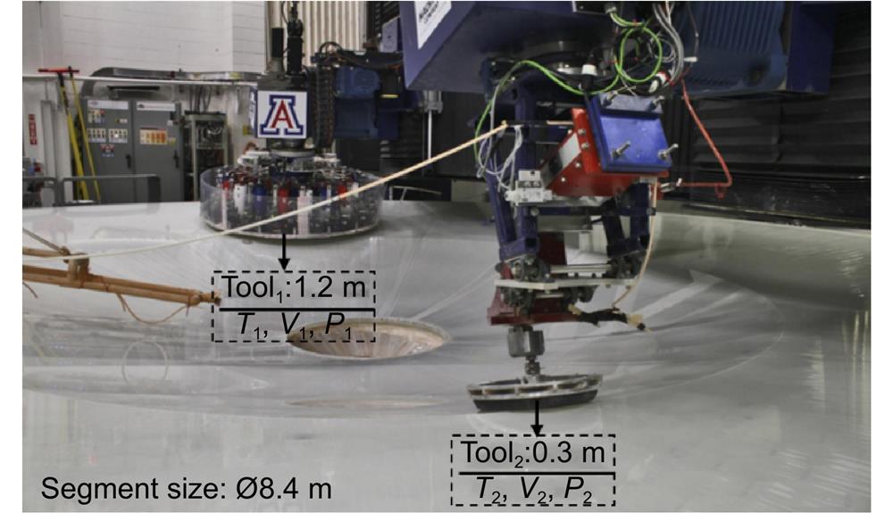
Fig. 1. Large polishing machine (LPM) with dual tools at the University of Arizona. Figure reproduced with permission from ref.⁶, Optical Society of America.

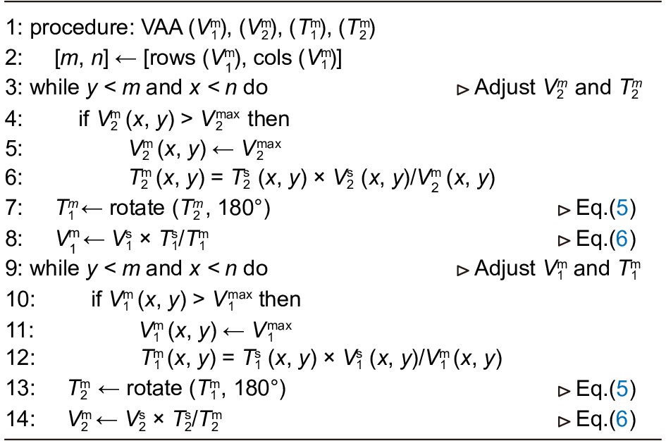
Fig. 2. Flow of velocity adjustment algorithm. Figure reproduced with permission from ref.⁶, Optical Society of America.

Fig. 3. The results of simulation: (a–b) two sequential single-tool runs using Tool₁ followed by Tool₂, (c) in-in feed with equal-angle path, (c) in-out feed with equal angle path, (d) in-in feed with equal-arc-length path, and (f) in-out feed with equal-arc-length path. Figure reproduced with permission from ref.⁶, Optical Society of America.

Fig. 4. Flow of RIFTA dwell time algorithm.

Fig. 5. (a) Initial surface error map from real measurement, (b−f) dwell time calculation results, and (g−k) estimated residuals in the CA without using RIFTA (b, g), adding γ optimization (c, h), adding inner iterations (d, i), adding outer iterations (e, j), and resampling to 1 mm (f, k).

Fig. 6. Two 8.4 m in diameter LBT primary mirrors and the science instruments between the two mirrors in the middle of the telescope structure. Figure reproduced from LBTO.

Fig. 7. Laser truss configuration on the LBT prime focus mode. Laser trusses extend from nine collimators around the primary mirror to three retroreflectors on the prime focus camera, with three collimators aligned to each retroreflector. Additionally, there are two nearly orthogonal channels to monitor the diameter of the mirror. Figure reproduced with permission from ref.¹¹, SPIE.

Fig. 8. (a) The ability of the TMS to measure pose was validated using commanded Rx motion on the primary mirror. (b) Horizontal and vertical first-order coma Zernike coefficients, produced using a perturbed LBT optical model, show the anticipated variability for on-axis and off-axis fields. Figure reproduced with permission from ref.¹¹, SPIE.

Fig. 9. Schematic presenting the major steps in transforming raw channel length measurements to a “change of pose” correction vector. The core functionality of the TCP/IP software lies in the shaded, starred box. Figure reproduced with permission from ref.¹², SPIE.

Fig. 10. (a) Optical layout of MOBIUS. Each MOBIUS module consists of a right-angle mirror, a spherical mirror as collimator, and a dispersing prism which is made of Strontium titanate (SrTiO₃). The incident beam from LBT will be deflected by the right-angle mirror near the focal plane. (b) As MOBIUS will utilize existing slit mask frame, it requires no modification to current LUCI hardware settings. Figure reproduced with permission from ref.¹³, SPIE.

Fig. 11. (a) Without MOBIUS, zJHK spectra are overlapped so filters are required to distinguish each band. (b) MOBIUS provides dispersion in the perpendicular direction (shown as in this diagram). As demonstrated, we can simultaneously obtain zJHK spectra simultaneously with 2.3 arcsecond of maximum slit length without overlap. Figure reproduced with permission from ref.¹³, SPIE.

Fig. 12. (a) Spot diagram at the LBT focal plane of K-band. The RMS radius of spot size is increased when MOBIUS is introduced. However, considering the expected spot size delivered by the telescope is 150 µm, the variation caused by MOBIUS is insignificant. (b) Ensquared energy diagram at the LUCI detector plane of K-band. Similarly, the variation induced by MOBIUS is negligible as the pixel size of detector is 18 µm. Figure reproduced from: (a) ref.¹³, SPIE; (b) ref.⁴², LUCI.

Fig. 13. (a) Pictures of fabricated MOBIUS optics elements. The size of optics is limited to fit in slit mask frame. (b) Modeling of the MOBIUS-installed frame. To compensate the added weight from MOBIUS, the frame has light-weighted features.

Fig. 14. A thin, circular arc obscuration with an angle of φ lying in the aperture plane is shown on the left. Such obscuration gives rise the “bow-tie/searchlight effect^{46, 49, 53}in the Fraunhofer diffraction pattern shown on the right.

Fig. 15. Illustration of the segmented pupil topologies studied in this session, and all of them have the same aperture diameter of 12 m and gap width of 20 mm. The reflectance of the pupil is color-coded with black and white, the white area is the reflecting surface (mirror), while the black one shows the obscured area. Figure reproduced with permission from ref.¹⁴, SPIE.

Fig. 16. The normalized PSFs of pupils in Fig. 15, subtracted with that of the circular pupil in Fig. 15(a), i.e. ideal Airy disk function. Note that every PSF is normalized to the peak value before the subtraction is performed.

Fig. 17. (a) Conceptual space deployment image of the Nautilus array in orbit. (b) A color-corrected MODE lens developed by the Nautilus team. (c) A molded Gen4 MODE lens prototype using low-temperature glass.

Fig. 18. (a) The assembled KEYS prototype. (b) A cross-section view showing the contact points of the ball bearings on the step-like features of the MODE lens. Figure reproduced with permission from ref.²⁰, SPIE.

Fig. 19. The real data from the metrology system. (a) Live view from the camera. (b) All segments are well-aligned against initial co-phasing status. The black line represents the actual size of the single segment. It measures the unobscured area (from the KEYS structure), which is large enough to sense and monitor the misalignment. (c) Segment 3 drifted from the reference position and the measured tilting angle is 0.006°. (The X and Y axis units of (b) and (c) are in pixels.) Figure reproduced with permission from ref.²¹, SPIE.

Fig. 20. Schematic diagram showing a mock-up MODE lens segment (i.e., Mock Lens Segment) mounted on the automatic KEYS adopting computer-controlled stepper motor actuators to make closed-loop orientation and position adjustments (i.e., alignment and co-phasing) to the mock-up MODE lens segments.

Fig. 21. Conceptual rendered image of the OASIS space observatory with a 20-metrer diameter inflatable primary aperture (yellow disk-like membrane on the right side of the image).

Fig. 22. A coarse tool such as a laser distance gauge can easily measure the longitudinal distance within 2 millimeters. The shape error sensitivity is vastly dominated by the lateral calibration errors ε_y or ε_x, which require 300 microns of accuracy to meet the global measurement requirement. Since the compact deflectometer head is portable and quasi-kinematically mounted, this can easily be achieved in an offsite coordinate measuring machine.

Fig. 23. A simulation showing inherent surface shape and instrument test error is provided. Sample test measurement 1 and 2 differ in that a rotated surface shape was added to the static instrumental error map to produce them. ‘Unrotating’ each of the six maps to the original unclocked positions produces an average that is remarkably similar to the true inherent surface shape. Taking the difference between this average and underlying inherent surface shape yields an error of less than 0.5% of the systematic error originating from the measuring instrument.

Fig. 24. (a) Front view of the inflatable 1-meter OASIS primary aperture prototype solid model. (b) The deflectometer head is mounted onto a telescope mount and features a typical machine vision camera, a high-quality LCD display, and a laser for alignment with the test mirror’s optical axis. The deflectometry assembly (LCD screen, laser, and camera) was affixed to an OPTRON telescope mount with 3 DOFs so alignment could be achieved between the mechanical axis of the OASIS 1-meter prototype and the calibrated center point of the deflectometer.

Fig. 25. The rendering image of the UV space telescope Hyperion examining the fuel for star formation by probing the nature, extent, and state of H₂ at the crucial atomic-to-molecular interstellar medium boundary layer^{25, 26}. Figure reproduced with permission from ref.²⁵, SPIE.

Fig. 26. The cross-dispersion spectroscopy optics layout (b) and beam footprint on the échelle grating plane (a). Figure reproduced with permission from ref.²⁵, SPIE.

Fig. 27. The diffraction efficiency calculation results for (a) échelle grating and (b) cross dispersion and (c) spectrum distribution on the 52 mm × 52 mm sensor plane. The three orders of the échelle grating are overlapped, but those are separated by cross dispersion horizontally on the sensor. The high-order of échelle grating dispersive the spectrum rapidly, and it implements the R >30000. Figure reproduced with permission from ref. ²⁵, SPIE.

Fig. 28. (a) Optomechanical rendering of the CDEEP optical configuration showing the unobscured SiC telescope and integrated optical bench. (b) Raytrace of the coronagraph optical train beginning at the secondary mirror M2. Figure reproduced with permission from ref.²⁷, SPIE.

Fig. 29. An expanded realization of the CDEEP testbed with two deformable mirrors to study a coronagraph’s ability to correct diffraction features that result from heavily segmented pupils (e.g., LUVOIR⁸⁶) or secondary support spiders (e.g., Nancy Grace Roman Space Telescope⁸⁷) using the Active Correction for Aperture Discontinuities technique⁸⁸.