Astronomical advances are largely coupled with technological improvements. From the invention of the first optical telescope used by Galileo in 1609 and through the foreseeable future, astronomy and optical engineering are forever linked. In this paper, several advances are summarized that will enable future telescopes to probe and expand our scientific understanding of the universe.

To begin, Section Deterministic computer controlled optical surfacing technologies covers optical fabrication and manufacturing process optimization technologies. Fabrication of large optics is an extremely time-consuming process due to the large size and high-accuracy requirements^1-4. For example, polishing each segment of the Giant Magellan Telescope (GMT) to the specified accuracy consumed about one year. Modern precision optical surfaces are manufactured with Computer Controlled Optical Surfacing (CCOS) processes^5-7, such as small-tool polishing^{5, 7}, bonnet polishing⁸, magnetorheological finishing, ion beam figuring^{9, 10}, etc. With these systems, there are two main categories of methods for improving polishing efficiency: increasing the material removal rate and minimizing the total dwell time. In this section, both categories are addressed. The mathematical theory of multiplexed two CCOS runs for simultaneous use of two polishing tools has been developed⁶. Dwell time optimization is demonstrated via Robust Iterative Fourier Transform-based dwell time Algorithm (RIFTA)⁹. These emerging technologies provide opportunity to increase speed and reduce cost of large optics manufacturing.

Section Very large telescope control system, instrument, and segmentation summarizes optical engineering technology developments for very large telescopes. As a first example, the Large Binocular Telescope (LBT) team is developing a laser-truss based alignment system for maintaining telescope collimation and pointing^{11, 12}. The laser truss metrology system, able to measure the relative position of optics in six degrees of freedom, is the first of its kind to be implemented on large, ground-based telescopes. A second innovation for the LBT system is an instrument package referred to as MOBIUS (Mask-Oriented Breadboard Implementation for Unscrambling Spectra). The MOBIUS system adds cross-dispersion capability to the existing LUCI (LBT Utility Camera in the Infrared) near infrared (NIR) imagers and spectrographs¹³. By inserting the MOBIUS module, we extend simultaneous coverage down to 0.32 µm by binocular observations with one MODS (The Multi-Object Double Spectrographs) and one LUCI. The final example discussed in Section Very large telescope control system, instrument, and segmentation is segmentation of primary mirror apertures. A pinwheel aperture segmentation is a promising approach which obtains a point spread function (PSF) with enhanced axial symmetry. This is modeled using Fraunhofer diffraction theory with the Python-based POPPY simulation tool¹⁴.

Section Future space telescope concepts and enabling technologies introduces some next generation space telescope concepts. The multi-order diffractive engineered (MODE) lens is a novel optical element that is lightweight, achromatic across a large spectrum and has more relaxed tolerances than mirror segments of a similar size^15-19. The Nautilus Space Observatory concept provides a new solution utilizing the transmissive MODE lens segments. Our group has developed both a mechanism to align MODE lens segments²⁰ and an in-process metrology system to monitor the lens alignment while the segments are being bonded together²¹. The Orbiting Astronomical Satellite for Investigating Stellar Systems (OASIS) is a proposed terahertz space observatory that will explore the role of water in the evolution of planetary systems and features a 20-meter diameter primary mirror, which is obtained by using inflatable membrane technology^{19, 22-24}. By pressurizing one transparent and one metallized membrane sealed around a rigid tensioning ring, a lenticular surface with immense light-collecting power can be obtained. We present a metrology technique for measuring the surface figure of such novel inflatable mirrors²⁴. At the other end of the optical spectrum, the next generation UV space telescope concept, Hyperion, is designed to examine the origin of the star formation^{25, 26}. At the atomic-to-molecular interstellar boundary layer, the fuel for star formation (SF) exists in a state of H2. Both the reflective telescope and cross-dispersion instrumentation design using freeform optics are presented. The Coronagraphic Debris and Exoplanet Exploring Pioneer (CDEEP) is a SmallSat mission concept for high-contrast imaging of circumstellar disks and exoplanets. CDEEP is equipped with a vector vortex coronagraph (VVC) to achieve the contrast necessary to resolve debris disks in scattered light at visible wavelengths (<10^-8 with post processing). This instrument will enable the classification of transport-dominated debris disks by measuring the albedo, composition, and morphology with extreme sensitivity. The design of the CDEEP mission and associated vacuum compatible high-contrast imaging testbed are documented in Maier et al²⁷.

The authors acknowledge that this invited summary paper is significantly based on and directly overlaps with many parts of a previous conference publication²⁸. The goal of this extended review article is to provide comprehensive details and substantial updates with additional/reorganized materials presenting the latest optical engineering technology developments conducted at the University of Arizona.

Fabricating the large, complicated optical surfaces required by future telescopes is continuously being improved with innovative techniques to reduce cost and time. In this section, two approaches are discussed. Simultaneous polishing with multiple tools of different sizes provides a holistic approach to polishing because tool size is related to the spatial frequency of the surface errors that can be corrected. The other method, dwell time optimization, improves the efficiency of the removal by spending more effort on the high surface and minimizing time spent in regions with low error. Both techniques help make future telescopes a reality.

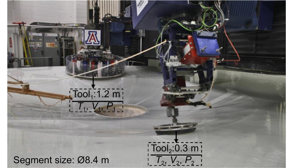
Many future telescope system designs utilize non-trivial optical surfaces and components such as freeform lens or mirrors in order to control the aberrations especially for wide field of view systems. Those precision optics manufacturing efficiency can be significantly improved if multiple fabrication tools are adopted simultaneously in a single polishing process. For instance, the Large Polishing Machine (LPM) in Fig. 1 consists of two tools with different sizes. A 1.2 m diameter stressed lap (labelled Tool₁) and a 0.3 m diameter non-Newtonian lap (labelled Tool₂) have been used in the LPM to ensure adequate removal for the Large Synoptic Survey Telescope (LSST) and GMT. They can be controlled simultaneously and independently during a single CCOS run.

In order to accelerate the polishing process speed, a dual-tool multiplexing polishing model enabling simultaneous running of the two polishing heads was developed⁶. The convolutional material removal model of an individual tool is defined as

$Z\left( {x,y} \right) = R(u,v) * * [T\left( {x,y} \right) \times V\left( {x,y} \right) \times P\left( {x,y} \right)]\;,$ (1)

where “**” represents the convolution operator; Z(x,y) is the removed material distribution, which is equal to the convolution between the basic Tool Influence Function (TIF) R(u,v) and the product of the dwell time T(x,y), the velocity V(x,y), and the contact pressures P(x,y). Equation (1) is still valid in the dual-tool multiplexing model. Moreover, since the material removed at a certain dwell point in the single-tool model is required to be identical to that in the dual-tool model, the following boundary condition BC (BC-1) should be fulfilled,

$\rm{BC-1} :{Z}_{1}^{\rm{s}}(x,y)\equiv {Z}_{1}^{\rm{m}}(x,y)\;\;\;{\rm{and}}\;\;\;Z_2^{\rm{s}}(x,y) \equiv Z_2^{\rm{m}}(x,y)\;, $ (2)

where $Z_1^{\rm{s}}\left( {x,y} \right)$ and $Z_2^{\rm{s}}\left( {x,y} \right)$ represents the material removed by R₁ (the basic TIF of Tool₁) and R₂ (the basic TIF of Tool₂) at $\left( {x,y} \right)$ in the single-tool model, respectively; $Z_1^{\rm{m}}\left( {x,y} \right)$ and $Z_2^{\rm{m}}\left( {x,y} \right)$ represents the material removed by R₁ and R₂ at $\left( {x,y} \right)$ in the dual-tool model, respectively. Since R₁ and R₂ remain invariant, Eq. (2) can be further transformed into

$\left\{\begin{gathered} T_1^{\rm{s}} \times V_1^{\rm{s}} \times P_1^{\rm{s}} = T_1^{\rm{m}} \times V_1^{\rm{m}} \times P_1^{\rm{m}} \\ T_2^{\rm{s}} \times V_2^{\rm{s}} \times P_2^{\rm{s}} = T_2^{\rm{m}} \times V_2^{\rm{m}} \times P_2^{\rm{m}} \\ \end{gathered}\;\right., $ (3)

where $T_1^{\rm{s}}$, $V_1^{\rm{s}}$ and $P_1^{\rm{s}}$ are the dwell time, the velocity, and the contact pressure of Tool₁ in the single-tool model, respectively; and $T_2^{\rm{s}}$, $V_2^{\rm{s}}$ and $P_2^{\rm{s}}$ are the dwell time, the velocity, and the contact pressure of Tool₂ in the single-tool model, respectively. Similarly, $T_1^{\rm{m}}$, $V_1^{\rm{m}}$, $P_1^{\rm{m}}$, $T_2^{\rm{m}}$, $V_2^{\rm{m}}$ and $P_2^{\rm{m}}$ are the corresponding parameters for Tool₁ and Tool₂ in the dual-tool model.

Since LPM works in workpiece rotation mode (see Fig. 1), the simultaneous run of the two tools requires the dwell time for each individual tool to be synchronized. This is achieved by setting one tool (e.g. Tool₁) as the primary tool so that its dwell time and velocities remain invariant, i.e.

$\left\{\begin{gathered} T_1^{\rm{s}}(x,y) = T_1^{\rm{m}}(x,y) \\ V_1^{\rm{s}}(x,y) = V_1^{\rm{m}}(x,y) \\ \end{gathered}\right.\;.$ (4)

In addition, during simultaneous polishing, Tool₁ and Tool₂ are placed at the opposite locations (i.e. 180°). Therefore, $T_2^{\rm{m}}$ can be calculated with the machine-specific BC (BC-2) as

$ {\rm{BC-2}}:{T}_{2}^{{\rm{m}}}(x,y)\equiv {\rm{rotate}}({T}_{1}^{{\rm{m}}}(x,y),180^ \circ ).$ (5)

It is worth mentioning that the separation angle between Tool₁ and Tool₂ can be arbitrary. The 180° is just the most convenient angle to implement the dual-tool model under LPM’s specific gantry-type configuration. Based on Eqs. (4) and (5), $V_2^{\rm{m}}$ is determined as:

$V_{\rm{2}}^{\rm{m}}(x,y) = V_2^{\rm{s}}(x,y)\frac{{T_2^{\rm{s}}(x,y)}}{{T_2^{\rm{m}}(x,y)}}.$ (6)

As the contact pressure is often set as constants, all of the parameters for the dual-tool model are now synchronized. However, $V_2^{\rm{m}}(x,y)$ obtained from Eq. (6) may exceed the maximum velocity allowed by the polishing machine. Therefore, the Velocity Adjustment Algorithm (VAA) shown by the algorithm in Fig. 2 is employed to constrain the velocities under the valid range. VAA adjusts the velocities of Tool₂ and Tool₁ in two loops, respectively. In the first loop, $V_2^{\rm{m}}(x,y)$ is clamped to the $V_2^{\max }$ if it is over the range, and $T_2^{\rm{m}}(x,y)$, $T_1^{\rm{m}}(x,y)$ and $V_1^{\rm{m}}(x,y)$ are updated accordingly. Similarly, in the second loop, $V_1^{\rm{m}}(x,y)$ is clamped to the $V_1^{\max }$ if it is over the range, and $T_1^{\rm{m}}(x,y)$, $T_2^{\rm{m}}(x,y)$ and $V_2^{\rm{m}}(x,y)$ are updated accordingly.

The performances of the single-tool sequential polishing and dual-tool simultaneous polishing are studied using a simulated surface error map in shown in Fig. 3, where Figs. 3(a) and 3(b) are the results of two sequential single-tool runs. The figure error is reduced from 1.72 μm RMS to 184.9 nm RMS after processed by Tool₁ (see Fig. 3(a)), which is then further decreased to 3.4 nm RMS by Tool₂ shown in Fig. 3(b). The total dwell time of the sequential runs is 22.62 + 36.54 = 59.16 h.

In the dual-tool multiplexed model, two tool-feed modes are tested, namely the in-out mode shown in Figs. 3(d) and 3(f) and the in-in mode shown in Figs. 3(c) and 3(e). The in-out mode is generally applicable to any dual-tool polishing scenario, because Tool₁ and Tool₂ move in the same direction and the tool collision can be avoided. The in-in mode has the potential problem of tool collision, however, it can also be applied for the GMT on-axis segment here, since this problem is automatically resolved because of the hole at the mirror’s center. Tool₁ is selected as the primary tool in the dual-tool polishing, so that the parameters of Tool₂ (i.e. the dwell time and velocities) are adjusted and synchronized with those of Tool₁. The performances of the in-in and the in-out feed modes are studied with equal-angel and equal-arc-length path types, respectively. With the equal-angel paths, as shown in Figs. 3(c) and 3(d), the in-in feed mode achieves 29.26 h, which is shorter than that (37.08 h) of the in-out feed mode. Compared with the single-tool sequential result, the polishing efficiency is improved by 50.54% with the in-in mode.

The two feed modes with the equal-arc-length paths are further demonstrated in Figs. 3(e) and 3(f). The total dwell time of the in-in feed mode shown in Fig. 3(e) is 29.26 h, which achieves a similar residual error as those in Figs. 3(c) and 3(d). It is worth mentioning that, however, the in-out feed mode cannot be applied with the equal-arc-length path as shown in Fig. 3(f), since the two tools have different redial positions at any instant so that the arc lengths cannot be equal.

In a word, the multiplexed dual-tool deterministic polishing model can enable the efficient polishing of large optics. Also, the dual-tool multiplexing model can be further extended to an N-tool model multiplexing N tools, in which case the polishing efficiency can be further improved.

One of the most essential numerical optimization problems of a CCOS process is to optimize the dwell time which controls how much time a tool dwells at a certain position on the surface of a workpiece. The dwell time optimization is guided by the convolutional polishing model²⁹,

$z\left( {x,y} \right) = b\left( {x,y} \right) * t\left( {x,y} \right)\;,$ (7)

where “ $ * $” represents the convolution operation, $b\left( {x,y} \right)$ is the Tool Influence Function (TIF), $z\left( {x,y} \right)$ is the removed material, and $t\left( {x,y} \right)$ is the dwell time. $z\left( {x,y} \right)$ and $b\left( {x,y} \right)$ are known, $t\left( {x,y} \right)$ is thus calculated via deconvolution, which is an ill-posed operation that may not result in a reliable and unique solution of $t\left( {x,y} \right)$. Equation (1) implies that, to achieve the desired figure in a Clear Aperture (CA), $t\left( {x,y} \right)$ should be optimized on a Dwell Grid (DG) which is larger than the outline perimeter of the CA with the radius of $b\left( {x,y} \right)$. A reliable $t\left( {x,y} \right)$ solution should fulfill three requirements. First, it should be non-negative, since CCOS techniques usually do not have the material adding capability. Second, it should minimize the estimated residual in the CA with the shortest total dwell time to guarantee the fabrication efficiency. Third, the computation time of $t\left( {x,y} \right)$ should be reasonable.

Three categories of dwell time optimization algorithms, namely the matrix-based algorithms^30-34, the Bayesian algorithm³⁵, and the Fourier transform-based algorithm³⁶, that partially fulfill these requirements have been attempted. The matrix-based algorithms modeled the deconvolution in an algebraic way, where $t\left( {x,y} \right)$ is solved from an over-determined linear system. Since the matrix is ill-conditioned and rank-deficient, $t\left( {x,y} \right)$ is always unsmooth, unless certain constraints are added^{32-34, 37}. However, the introduction of constraints makes the linear system much more complicated which cannot be efficiently solved when the measurement scale is large. The Bayesian algorithm³⁵ assumes a Poisson distribution of $t\left( {x,y} \right) * b\left( {x,y} \right)$ and a uniform distribution of $z\left( {x,y} \right)$, from which $t\left( {x,y} \right)$ is solved via the Richardson-Lucy algorithm³⁸. This algorithm automatically guarantees the non-negativity of $t\left( {x,y} \right)$, however, it contains a regularization hyper-parameter, which is hard to tune in practice. The Fourier transform-based algorithm³⁶ is very computationally efficient since deconvolution is transferred to pointwise division in frequency domain by the Fast Fourier Transform (FFT) algorithm as

$t\left( {x,y} \right) = {F^{ - 1}}\left[ {\frac{{{Z_{\rm{d}}}\left( {u,v} \right)}}{{B\left( {u,v} \right)}}} \right],$ (8)

where “ ${F^{ - 1}}$” represents the inverse Fourier transform, ${Z_{\rm{d}}}\left( {u,v} \right)$ is the Fourier transform of the desired removal on the dwell grid, i.e.${z_{\rm{d}}}\left( {x,y} \right)$, and $B\left( {u,v} \right)$ is the Fourier transform of the TIF $b\left( {x,y} \right)$. However, the close-to-zero frequencies during the division may amplify the noise and a thresholded inverse filtering step is introduced as

$t\left( {x,y} \right) = {F^{ - 1}}\left[ {\frac{{{Z_{\rm{d}}}\left( {u,v} \right)}}{{B\left( {u,v;\gamma } \right)}}} \right],$ (9)

where γ is the threshold value and

$B\left( {u,v;\gamma } \right) = \left\{ \begin{gathered} B\left( {u,v} \right),\,\,\,\,\,\,\left\| {B\left( {u,v} \right)} \right\| > \gamma \\ \gamma ,\,\,\,\,\,\,\,\,\,\,\,\,\,\,\,\,\,\,\,{\rm{otherwise}} \\ \end{gathered} \right..$ (10)

This threshold value again, becomes a hyper-parameter that is usually chosen by trial-and-error.

Based on the Fourier transform-based algorithm, we proposed a Robust Iterative Fourier Transform-based dwell time Algorithm (RIFTA)⁹ that fulfills all the three characteristics of dwell time mentioned above while maintains FFT’s high computational efficiency. First, the Nelder-Mead algorithm³⁹ was employed to directly search the optimal threshold γ for the thresholded inverse filtering. Second, a two-level iterative scheme was proposed to guarantee the non-negativity of the dwell time with the minimal increase in the total dwell time. Third, bicubic resampling was introduced to flexibly adapt the calculated dwell time to any machining intervals in a real CCOS process. The algorithm flow of RIFTA is given in Algorithm 1, which is briefly explained in the followings. Details of RIFTA can be found in ref.⁹.

Finding the optimal γ. We define a residual map ${z_{\rm{r}}}$ to be the difference between the desired removal ${z_{\rm{d}}}$ and the removed material $z\left( {x,y} \right)$ as

${z_{\rm{r}}} = {z_{\rm{d}}} - z\;.$ (11)

The effectiveness of $t\left( {x,y} \right)$ can ben quantitatively evaluated by interrogating the Root Mean Square (RMS) of ${z_{\rm{r}}}$ as $RMS\left[ {{z_{\rm{r}}}} \right]$. The optimal γ can be found from an unconstrained optimization problem as

${\gamma _{\rm {opt}}} = \mathop {\arg \min }\limits_\gamma RMS \left[ {{z_{\rm{r}}}\left( {x,y} \right)} \right].$ (12)

Substituting Eqs. (7), (9) and (11) to Eq. (12), the optimization objective can be reformulated as

$\begin{split} &{\gamma _{\rm{opt}}} = \\& \mathop {\arg \min }\limits_\gamma {\rm{RMS}} \left\{ {{z_{\rm{d}}}\left( {x,y} \right) - b\left( {x,y} \right) * {F^{ - 1}}\left[ {\frac{{{Z_{\rm{DG}}}\left( {u,v} \right)}}{{B\left( {u,v;\gamma } \right)}}} \right]} \right\}.\end{split} $ (13)

It can be observed that the optimization space in Eq. (13) is not smooth due to the thresholding and cropping operations. Its gradients thus cannot be calculated so that any derivative-based optimization algorithms can hardly be applied. In RIFTA, as shown in Line 8 in the RIFTA algorithm in Fig. 4, the Nelder-Mead algorithm is applied to directly search ${\gamma _{\rm{opt}}}$. The initial guess ${\gamma _{\rm{ini}}}$ is obtained as the ratio between ${\rm{RMS}}\left[ {{z_{\rm{d}}}} \right]$ and ${\rm{RMS}}\left[ {{z_{\rm{r}}}} \right]$ when $\gamma = 1$.

Two-level iterative scheme. If the smallest entry of ${z_{\rm{d}}}$ is outside the CA, to ensure the non-negativity of $t$, a constant piston should be added to offset the smallest entry in the DG. This operation, however, will inadvertently increase the total dwell time. Therefore, in RIFTA, as shown by Lines 6 – 16 in Algorithm (Fig. 4), the inner iterations only depend on the residuals in the CA, i.e ${z_{{\rm{r\_ca}}}}$, to adjust the pistons in the DG. In each iteration, ${z_{\rm{d}}}$ is only offset by a piston of $min\left( {{z_{\rm{r\_ca}}}} \right)$, where $min\left( \cdot \right)$ represents the minimum entry in “ $ \cdot $”. The negative entries in the calculated $t$, as shown in Line 9, are set as zeros in Line 10. In this way, ${z_{\rm{d}}}$ is always guaranteed to be adjusted by the smallest pistons during the iterative updates. As shown in Line 15, these inner iterations are performed until the Standard Deviation (STD) of the difference between the current and the previous residuals in the CA is less than the threshold std_t or the maximum number of iteration max_it is reached. The outer iterations are then added to tune the size of the DG, since we found that a much smaller DG is sufficient to obtain the desired ${z_{\rm{r\_ca}}}$ while the total dwell time is significantly reduced. As shown in Algorithm 1, starting from $s = \left\lfloor {{r_b}/2} \right\rfloor $, the outer iterations keep searching for the smallest s that fulfills the same stopping criteria as the inner iterations.

Bicubic resampling. To enable the flexibility of having different sampling intervals between metrology and fabrication hardware, we use bicubic resampling to downsample t to any required machining intervals that a CCOS process requires. As shown in Fig. 5, the algorithmic accuracy is not affected by this resampling scheme.

The performance of RIFTA is evaluated on real measurement data shown in Fig. 5(a), where a rectangular flat mirror is measured with 0.12 mm sampling interval using the sub-aperture stitching interferometry platform^{40, 41}. The size of the CA is set as 200 mm × 5 mm. The initial figure error in the CA is 167.02 nm Peak-to-Valley (PV) and 38.39 nm RMS. We use a Gaussian TIF with the peak removal rate of 1 nm/s and a radius of 5 mm so that the initial DG size is 210 mm × 15 mm.

Figures 5(b−f) shows the different dwell time calculation results. The corresponding estimated residuals in the CA are given in Figs. 5(g−k). Without using RIFTA, as shown in Figs. 5(b) and 5(g), the total dwell time is 3411.32 mins while the residual in the CA remains at 8.44 nm RMS using ${\gamma _{\rm{ini}}} = 1.6709 \times {10^6}$, which indicates that the calculated dwell time is far from the optimal solution. After γ is optimized as ${\gamma _{\rm{opt}}} = 1.6650 \times {10^6}$, the RMS of the residual in the CA reduces to 0.47 nm as shown in Fig. 5(h). The total dwell time shown in Fig. 5(c) is similar to that in Fig. 5(b). Afterwards, the inner iterations are employed to shorten the dwell time. Fig. 5(d) shows that the inner iterations bring the total dwell time down to 584.28 mins with an equally good residual in Fig. 5(i). As shown in Figs. 5(e) and 5(j), the dwell time is further reduced to 479.08 mins after the outer iterations for the DG size optimization. The minimized DG size is 207.4 mm × 12.6 mm. The final dwell time, as shown in Fig. 5(f), is obtained by down-sampling Fig. 5(e) to 1 mm sampling interval by bicubic resampling. The final estimated residual in the CA shown in Fig. 5(k) is not affected by the resampling operation, which proves that RIFTA is an effective dwell time optimization algorithm for CCOS processes.

Large, ground-based telescopes dominate modern astronomy. The heritage and lessons learned from these systems create the foundations for future telescopes. In this section, three areas are discussed. The first two, alignment system and cross-dispersion science module, will enable the Large Binocular Telescope (LBT) to produce new and more accurate astronomical observations. The third topic proposes design improvements to telescope mirror segmentation and secondary mirror obscurations created by the support structures.

The Telescope Metrology System measures changes in distance between various points around the primary mirror and retroreflectors fixed to the prime focus camera (LBC), forming a system of laser trusses to determine the “pose” (relative positioning and orientation) of the primary mirror shown in Fig. 6 to LBC prime focus configuration. Each laser truss consists of measurement arms extending from collimators positioned around the primary mirror cell to retroreflectors on the LBC, as shown in Fig. 7. An absolute distance measuring interferometer, the Etalon Absolute Multiline Technology (EAMT), measures laser truss leg lengths with micron-level accuracy over a 10 meter baseline about once every ten seconds. To determine the pose of the optical elements, an inverse kinematic analysis based on the Stewart-Gough hexapod platform is performed on laser truss lengths. With the pose computed, necessary positioning and rotation corrections may be commanded on the primary mirror to improve collimation and pointing.

The ability of the TMS to measure the relative position and orientation of the primary mirror was validated using incremental motion commanded on the primary mirror, spanning the full range of motion for normal telescope operation. Results for measured Rx motion are presented in Fig. 8. The maximum deviation between the calculated pose and the telescope controls was 1.7 µm in lateral motion (X, Y, Z) and 0.1 arcsec in rotational motion (Rx, Ry, Rz), which are within the expected range of deviation given the TMS measurement accuracy.

To further verify the validity of the TMS functionality, measured primary mirror position and orientation data were incorporated into an optical model for optical aberration and image quality analysis. For commanded rotations about X, or Rx motion, Zernike coefficients for both horizontal and vertical first-order coma were determined as shown in Fig. 8. Both on-axis and off-axis fields were considered in this analysis, where the field was increased parallel to Z7 horizontal coma. The anticipated field-dependence is exhibited in Z7 magnitude at off-axis field positions. Vertical coma, Z8, exhibits no field-dependence with primary mirror Rx rotation as the aberration is oriented perpendicular to the increase in field. Primary functionality of the TMS has been successfully demonstrated at prime focus for monocular mode¹¹.

The Telescope Metrology System has begun transitioning from “concept testing” and prototyping on LBT to implementation as an integrated part of the Telescope Control System (TCS)¹². As such, emphasis has shifted from solely focusing on accuracy to include system reliability and error handling. In its simplest possible configuration, the TMS consists of nine metrology channels from the right side (DX) primary mirror to three retroreflectors on the LBC red channel. Various system attributes are undergoing refinement during this stage, including: upgrading collimator optics and mount; implementing optical path difference (OPD) corrections to vacuum length; implementing inverse kinematic pose calculations; implementing software error handling; and developing robust and reliable software interaction with the metrology system and telescope.

Achromatic fiber collimators are critically important when using the EAMT system. For monochromatic collimators, the metrology waveband (1532 +/– 70 nm) and the alignment waveband (633 nm) produce very different beam diameters at a distance of 10 meters. To combat this problem, an achromatic collimator was designed to mitigate alignment difficulty. Larger diameter collimators are also being standardized for the TMS, as they improve the beam-walk tolerance and increase the contrast interference signals, improving overall robustness. Besides hardware improvements, enhancements to system calibration in software the OPD of the laser truss path length varies with temperature, pressure, humidity, and CO₂ content, with the temperature contribution presenting the dominant effect. Utilizing telemetry from the observatory sensors, Ciddor corrections are applied to optical path length to perform a “vacuum” correction.

To improve the robustness and error handling capabilities of the TMS, the LBTO software group has implemented an TCP/IP (transmission control protocol/internet protocol) software interface, enabling network communication to the EAMT unit via the TCP server¹². An experimental code has been developed to take measurements, manage interactions between the metrology system and the telescope, and send pose-corrections to the primary mirror. The core functionality of this code is focused on transforming raw channel length measurements to a final “change of pose” vector, which is first adjusted for various telescope instrument offsets, then sent to the TCS as the final correction vector. A schematic outlining the primary functional components of the TMS software is shown in Fig. 9.

First, a pose vector is computed from raw lengths received. Then we subtract the most recent reference pose, the pose measured following the last active-optics cycle using Focal Plane Image Analysis (FPIA). The change of pose is then further processed to combine various terms such as prime focus camera guiding corrections, PSF instrument offsets, as well as primary mirror bending terms, etc. to obtain the final correction to send to TCS. Following some pending requirements review and on-sky commissioning, we are nearly ready to deploy the software for routine use on the LBT.

Currently, the TMS team is working to produce a comprehensive hardware and software metrology package to support ongoing LBC operations. The system has proven successful in passive tests, running in parallel with science observations without sending corrections. Next, the system must complete on-sky commissioning during telescope engineering time. The key benchmarks that the TMS must meet are reliability, accuracy, and operability.

The MOBIUS (Mask-Oriented Breadboard Implementation for Unscrambling Spectra) is a plug-in module (Fig. 10) which will be placed at the focal plane of LBT to provide cross-dispersion for LUCI¹³. This module disperses the input slit images in the perpendicular direction to the existing grating to cover zJHK bands simultaneously (Fig. 11) with a single LUCI. As every optical element will be installed inside of current LUCI’s slit mask frame, using MOBIUS requires no modifications in current instrument settings. Since MOBIUS consists of two identical cross disperser modules, it will also provide sky subtraction by dithering between source and sky position.

A key optical requirement of MOBIUS is retaining image quality despite the insertion of the module. To verify that the image quality is not degraded, we compared the RMS spot radius at the focal plane of the LBT and the ensquared energy at the detector plane (Fig. 12). From simulations, the RMS spot radius increased in every band after MOBIUS was introduced, however, this spot is still smaller than the expected size delivered from the telescope, which is 150 µm at focal plane. (Fig. 12(a)) Further, the greatest difference in half width distance for 90% fraction ensquared energy is also about 2 µm which is smaller than a pixel size of detector which is 18 µm (Fig. 12(b)). These results demonstrate that the MOBIUS can expand wavelength coverage of a single LUCI while generating negligible variation in optical performance.

Currently the MOBIUS optics elements are fabricated (Fig. 13(a)) and frame modeling for prototype is done (Fig. 13(b)).

As early as 1941⁴³, Werenskiold, an amateur astronomer and telescope builder has recorded that curved spiders on secondary mirror could greatly improve the quality of the planetary observation, followed by similar experimental results from Couder (1952)⁴⁴ and Everhart and J. Kantorski (1959)⁴⁵. Until 1984, Richter⁴⁶ provided a detailed Fraunhofer diffraction calculation mathematically and proved that a thin, circular arc obscuration with an angle of φ lying in the aperture plane can spread out the flares with the same angle φ in the both sides in the diffraction patterns, shown in Fig. 14.

The previously-mentioned research^43-45, the secondary mirror spiders from Harvey and Ftaclas (1995)⁴⁷, apodized pupils with spatially varying transmission functions⁴⁸, and the diffraction noise caused by straight edges and gratings of hexagonal segment topology⁴⁹ indicated that the curved-sided segments might be a good alternative for future large telescopes design. Comparing to the high-contrast imaging systems with hexagonal segmented design and delicate instrument for current and future ground- and space-based telescopes⁵⁰, Breckinridge suggested a KISS (Keep It Simple for Space) rule with pinwheel pupil concept for space telescope design⁵¹. Such concept can reduce the number of optical surfaces, reduce the complexity (active wavefront control or apodized aperture) of the overall system, and then further reduce the cost for future mission. In 2018, Breckinridge and Harvey summarized the previous work, and proposed a pinwheel pupil solution⁴⁹ with digitally simulated results showing without narrow continuous flares and spikes⁵².

In this section, we compare the point spread function (PSF) of a pinwheel pupil (curved edges) and that of a keystone pupil (straight edges) and further illustrate how the curvature of the spokes in the pinwheel pupil plane can impact the PSF in the image plane. The discrete matrix Fourier Transform analysis is performed by Physical Optics Propagation in Python (POPPY)^{53, 54}, a Python library primarily developed by a team of astronomers at the Space Telescope Science Institute. The investigated pupils are shown in Fig. 15, and they are circular, circular with central obscuration, keystone, Pinwheel 180, Pinwheel 360, and Pinwheel 540 pupil. The numerical number indicated after each pinwheel pupil is the total degree of the curved spokes, in order to meet the bow-tie/searchlight effect spreading the light in 360 degree effect^{46, 49, 53}, following the pinwheel pupil prescription from Breckinridge and Harvey⁵². The normalized PSFs are calculated by POPPY. Fig. 16 shows the subtracted PSFs, which means that every normalized PSFs are subtracted by the normalized PSF of the circular aperture (Fig. 15(a)). By doing so, one can easier to observe directly what the footprint can the obscurations, the curved spokes in the pupil plane create in the image plane.

Figure 16(a) shows nothing because the PSF of the circular aperture is subtracted by itself. When the central obscuration is added, Fig. 16(b) illustrated that the energy among the concentric rings. In Fig. 16(c), the segment gaps and straight spokes are added to the aperture plane (Fig. 15(c)), and the consequences are the redistribution of the energy among rings and the straight flares in the PSF. The subtracted PSF of Pinwheel 180 shown in Fig. 16(d) indicates that the curved spokes can redistribute the straight flares along the rings, which is like spreading the beads on the rings, and this is called the “beading effect²⁸. More and more curvature of the spokes was added from Pinwheel 180 (Fig. 15(d)), Pinwheel 360 (Fig. 15(e)), and Pinwheel 540 (Fig. 15(f)), and one can observe that the beads are spread out azimuthally following the same direction of the bending of the spokes. Such effect can prevent the straight flares spanning radially across from the center to the outer rings. As a result, the PSF approaches more like an Airy Disk. The tolerance analysis⁵³ was presented for the pinwheel pupil. It was illustrated that the pinwheel pupil has low sensitivity in edge error⁵³, rotation error, and displacement error.

The pinwheel pupil solution can provide an Airy Disk-like PSF with stable performance with the manufacture and alignment error. The fundamental analysis presented in this section is participated to illustrate the advantages of the pinwheel pupil topology. Further investigation including system integration with optimized coronagraphs (e.g., Ruane et al 2018⁵⁵ and N’Daiye et al 2016⁵⁶) for exoplanet imaging remains to be studied. From the perspective of manufacturing and the KISS rule⁵¹, the benefit of using a pinwheel pupil provides an innovative solution creating a stable, Airy Disk-like PSF pattern, which can be a great alternative for future space/ground telescope missions.

Astronomers have long desired space telescopes which are free from the many limitations imposed by Earth’s atmosphere. To make these future telescopes practical, three new technologies are discussed. First is a discussion of new segmented lens alignment technology designed for exoplanet spectroscopy. The second topic addresses the limited launch capabilities of current rockets by proposing an inflatable primary mirror for terahertz OASIS telescope. As might be imagined, an inflatable mirror has unique metrology requirements. Also, this section introduces a novel space telescope design with cross-dispersed spectroscopy improvements for a far UV observation. Finally, this section reviews the CDEEP VVC coronagraph concept including an off-axis primary mirror and a microelectromechanical system (MEMS) deformable mirror (DM). To accurately simulate the incredibly sensitive performance in a relevant space-like environment, a vacuum compatible testbed has been designed to prototype and develop the coronagraph.

The Nautilus space observatory for exoplanet spectroscopy utilizes segmented transmissive lenses called MODE lenses as shown in Fig. 17. The alignment tolerances of a segmented MODE lens are on the order of micrometers rather than nanometers. The MODE lens is a novel, lightweight optical component that utilizes both a multi-order diffractive (MOD) lens and a diffractive Fresnel lens (DFL) surface to make a refractive optic that is significantly achromatic and lighter than a typical lens of similar optical power⁵⁷. Its light weight allows for its use in applications such as space observatories. The Nautilus space observatory is one such proposed observatory that would be used for exoplanet spectroscopy and would utilize a segmented MODE lens¹⁵.

A MODE lens is preferable to a reflective optic in this application because it has much looser alignment tolerances. However, new alignment technologies are still needed to reach these tolerances and meet engineering requirements specific to the MODE lens such as an unobscured aperture for use while bonding the lens segments. To enable the MODE lenses use in such a segmented primary, we have been developing an alignment technology called the Kinematically Engaged Yoke System (KEYS) shown in Fig. 18²⁰. KEYS utilizes ball-bearings to kinematically contact the MODE lens at the step-like features on the front MOD surface of the lens. This constrains the lens in five degrees of freedom, leaving rotation about the optical axis unconstrained. These ball bearings are attached to set screws, allowing for adjustment of tip, tilt and piston of the lens segments. Two of the setscrews are mounted on folded flexures which allow for two degrees of freedom of adjustment in the transverse plane.

A prototype KEYS was tested on a 240-mm, segmented PMMA MOD lens (no DFL). Our alignment was tested using a deflectometry measurement system and a ZYGO scanning white-light interferometer (SWLI). Using the SWLI, we were able to align segments within 20 microns which is within our tolerances for optical performance and our deflectometry system showed we had a tilt adjustment resolution of 0.006° as shown in Fig. 19²¹.

However, it has become necessary to adjust the lens while testing optical performance in order to be able to compensate for errors made during molding of glass MODE lens segments. In order to accomplish this, we are developing an automatic KEYS that uses actuators rather than manual set screws to make orientation and position adjustments to the lens segments. A stepper motor is coupled to a fine-thread setscrew using a flexible, helical coupling. To achieve finer resolution, those set screws push on lever flexures that have ball bearings adhered to them in order to kinematically contact the lens segment as shown in Fig. 20.

The Orbiting Astronomical Satellite for Investigating Stellar Systems (OASIS) is a 20-meter class space observatory that uses an inflatable membrane primary as shown in Fig. 21. Some challenges to measuring the specular concave surface include its large size, manufacturing variations such as wrinkles, and intentional but possibly large variations from annealing⁵⁸.

Deflectometry is well-posed to meet these metrology challenges because it is able to measure specular surfaces and can be reconfigured to measure a vast range of surface slopes, such as those produced at various inflation pressures^{59, 60}. The principal challenge to deflectometry in achieving global accuracy has historically been geometric calibration, but testing at a long distance lends the ability to achieve the required $\lambda /8\approx 67.5 \;{\rm{μm}}$ accuracy by using a portable deflectometer head that is calibrated offsite and aligned to the test surface in-situ²⁴.

Measurement uncertainty in the calibration of the system components, such the camera, test surface, and spatial light source, $\stackrel{\rightharpoonup}{{r}_{\rm{c}}},\stackrel{\rightharpoonup}{{r}_{{\rm{m}}}},$ and $\stackrel{\rightharpoonup}{{r}_{{\rm{s}}}}$, introduces different shape errors. Defining the direction $ \widehat{z} $ as parallel to optical axis of the nominally rotationally symmetric surface, axial miscalibrations along $ \widehat{z} $ produces radially symmetric error such as excess defocus or spherical terms, while lateral miscalibrations in the $ \widehat{x} $ or $ \widehat{y} $ directions embed excess astigmatism or higher order asymmetric error into the obtained measurement shape⁶¹.

Exploring deflectometry for a 1-meter OASIS primary antenna model, we show that the required calibration error by an external measurement device is relatively relaxed in the axial direction. At a measurement distance approximately equal to the radius of curvature (~4 m) in the inflated f/2.2 configuration, an uncertainty $ {\epsilon }_{z} $ within a bilateral 3.5 mm envelope is sufficient to produce the desired $ \lambda /8 $ measurement accuracy specification, shown in Fig. 22. Because the scale of the optical test setup (meters) dwarfs the uncertainty of the calibration measurement devices (millimeters), excess rotationally symmetric induced errors are not as nefarious in a long-distance deflectometer as they have been in smaller testing configurations.

As for errors induced by lateral calibration uncertainty, induced asymmetric shape can be removed using the N-Rotations methodology, familiar in the absolute interferometry literature⁶². The central thesis of these methods is that a measurement consists of inherent surface shape and spurious shape imbued by systematic calibration error. While the true surface shape rotates if the optic is physically clocked, the systematic calibration error does not. If measurements of a clocked optic are digitally unrotated and then averaged, rotationally asymmetric terms can be precisely cancelled out. Fig. 23 demonstrates this concept by simulating an inherent test shape and systematic error (in mm), measurements of the clocked optic, and the asymmetric term removal result. A clocking uncertainty of 0.5 degrees is added into the 6-rotation simulation to demonstrate its efficacy even with physical rotation stages.

Combined, the OASIS deflectometer concept is less susceptible to induced rotationally symmetric errors because of its long-distance testing configuration and its ability to rotate coaxially about the antenna’s optical axis. The 1-meter prototype configuration (Fig. 24) is used in scaling studies of the inflatable membrane architecture over a large range of pressures and up to the 20 m scale version.

Hyperion space mission (Fig. 25) targets the observation of Far Ultraviolet (FUV) spectral range where its investigation reveals the secret of the first stage of the star formation^63-65. Due to the spectrum complexity and population within the interesting FUV range (1405 Å – 1645 Å, 1 Å = 10^–10 m), the high spectral resolution spectroscopy with a wide field of view is an essential specification. The astronomer demand drives the optical design goal to achieve 5 arcsec spatial resolution, 10 arcmin instantaneous field of view, and greater than 30000 spectral resolution (R = λ/Δλ).

In order to meet the optical performance requirements, we adopted the extreme aspect ratio long-slit (240 aspect ratio, 10 arcmin × 2.5 arcsec) on the Ritchey-Chretién telescope. The hyperbolic mirrors for primary and secondary are designed to have the 2,400 mm effective focal length, and it passes the F/6 beam to spectroscopic apparatus^{25, 26}. The extreme aspect ratio of the long-slit and the high spectral resolution requirement (R > 30,000) at the FUV spectral range makes the Hyperion's optical design unique. The conventional spectrometer optical layout (off-axis collimator-grating-imaging optics) induces the significant aberration, especially when the long slit has to be installed into the high-resolution spectroscopy. We introduced the novel on-axis layout applying the collimation mirror on-axis through the center hole of the first grating (échelle grating), and the freeform imaging mirrors are embodied ( Fig. 26). The elliptical center hole on the échelle grating is designed to have zero photon loss by matching the secondary mirror's obstacle as shown in Fig. 26(a).

The on-axis layout of the primary mirror – secondary mirror – tertiary mirror – first grating (échelle) gives the minimized the field aberration along the slit length^{66, 67}. Moreover, the in-plane layout of the first grating (échelle) – cross dispersion grating – two freeform mirror – detector allows us to estimate and handle the aberration easily. Since the cross dispersion divergence angle after both gratings is large, the formation of the two freeform mirrors and surfaces are optimized based on the previously reported Type-4 design form approach⁶⁸. Once the optical design is selected, the diffractive performance is evaluated for the entire spectral range. Even though the geometric optical optimization carefully selects the grating diffraction order and line density, it doesn’t confirm the spectral efficiency. Furthermore, because the high-order échelle grating has a delicate spectral sensitivity, the diffraction efficiency simulation is an essential procedure. Based on the electromagnetic wave propagation simulation, both gratings’ blaze angles are determined to have the best efficiency at the targeting order as shown in Fig. 27.

The Coronagraphic Debris and Exoplanet Exploring Pioneer (CDEEP) is a SmallSat mission concept developed by the UArizona Space Astrophysics Laboratory in collaboration with the Large Optics Fabrication & Testing group. As a coronagraphic instrument which blocks on-axis starlight to allow detection of dim circumstellar debris disks, CDEEP is proposed to be a monolithic silicon carbide (SiC) three-mirror telescope and coronagraph instrument featuring a 34.9 cm primary mirror as shown in Fig. 28. This SmallSat design also serves as a technical pathfinder for future space coronagraph telescopes utilizing even larger monolithic mirror apertures⁶⁹. CDEEP leverages heritage from the Deformable Mirror Demonstration Mission (DeMI)^70-71, the PICTURE series balloon⁷² and sounding rocket missions^73-75, EXCEDE laboratory testing^{76, 77}, SiC optics^{78, 79} and the vast theoretical and experimental work conducted toward the development of VVC technology^80-83. The off-axis fore-optics eliminate problematic diffraction features from secondary mirror supports that would otherwise make high-contrast imaging more challenging. The fast Cassegrain objective feeds light to the fast-steering mirror (FSM) for pointing correction, and then to the DM for static and dynamic aberration correction. The corrected light is then imaged onto the VVC which rejects on-axis starlight while passing light from a debris disk and/or planet unperturbed. The rejected starlight is vignetted by a reflective Lyot stop and fed to the low-order wavefront sensor, while the light from the target of interest is passed to the science camera suite⁸⁴. With post-processing, the CDEEP coronagraph will achieve contrast levels of 10^–8, enabling the direct detection of debris disks and exoplanets²⁷.

To prototype this mission and develop a platform for exploring future high-contrast imaging concepts, a vacuum-compatible testbed based on the optical layout of CDEEP (Fig. 29) is under construction at the University of Arizona. This testbed will serve as the primary platform for testing the CDEEP mission concept, as well as investigations into VVC technology and electric field conjugation focal plane wavefront sensing⁸⁵. The high-performance and compact form factor are ideal for prototyping future high-contrast imaging instrumentation intended for spaceborne observatories. Presently, the optical and mechanical design of the testbed are completed, and construction is slated to begin in 2021. The testbed will begin operations in a cleanroom environment, but ultimately be integrated into a vacuum chamber for further testing and refinement in a relevant environment. The development of the CDEEP testbed marks the beginning of The University of Arizona’s journey to developing high-performance optical satellite payloads in support of space astrophysics and planetary science investigations.

A diverse selection of ground-based and space-based future telescope technologies are actively being conceptualized, designed, prototyped, and demonstrated at the University of Arizona. Optical polishing enhancements discussed in Section Deterministic computer controlled optical surfacing technologies enable efficient production of future optical elements. New engineering technology in Section Very large telescope control system, instrument, and segmentation will upgrade and expand capabilities of existing very large ground-based or space telescopes. Finally, in Section Future space telescope concepts and enabling technologies, a view of the future shows how space-based telescopes that had previously been only a dream, are now realizable through the advances in optical engineering technologies. This suite of optical technologies serves the next generation of astronomical investigations by offering novel yet applicable approaches that the wider design and engineering community can practically use. It is our hope that these contributions in design and instrumentation will not only provide new practical benchmarks for modern astronomy today, but also precipitate the next great insights and questions about our universe.

References

[1] HM Martin, RG Allen, JH Burge, DW Kim, JS Kingsley et al. Fabrication and testing of the first 8.4-m off-axis segment for the Giant Magellan Telescope. Proc SPIE, 7739, 77390A(2010).
[2] HM Martin, RG Allen, JH Burge, DW Kim, JS Kingsley et al. Production of 8.4m segments for the Giant Magellan Telescope. Proc SPIE, 8450, 84502D(2012).
[3] HM Martin, JH Burge, JM Davis, DW Kim, JS Kingsley et al. Status of mirror segment production for the Giant Magellan Telescope. Proc SPIE, 9912, 99120V(2016).
[4] HM Martin, R Allen, V Gasho, BT Jannuzi, DW Kim et al. Manufacture of primary mirror segments for the Giant Magellan Telescope. Proc SPIE, 10706, 107060V(2018).
[5] DW Kim, SW Kim, JH Burge. Non-sequential optimization technique for a computer controlled optical surfacing process using multiple tool influence functions. Opt Express, 17, 21850-21866(2009).
[6] XL Ke, TY Wang, H Choi, W Pullen, L Huang et al. Dual-tool multiplexing model of parallel computer controlled optical surfacing. Opt Lett, 45, 6426-6429(2020).
[7] DW Kim, WH Park, SW Kim, JH Burge. Edge tool influence function library using the parametric edge model for computer controlled optical surfacing. Proc SPIE, 7426, 74260G(2009).
[8] VS Negi, H Garg, Kumar Shravan, V Karar, UK Tiwari et al. Parametric removal rate survey study and numerical modeling for deterministic optics manufacturing. Opt Express, 28, 26733-26749(2020).
[9] TY Wang, L Huang, H Kang, H Choi, DW Kim et al. RIFTA: a robust iterative Fourier transform-based dwell time Algorithm for ultra-precision ion beam figuring of synchrotron mirrors. Sci Rep, 10, 8135(2020).
[10] TY Wang, L Huang, Y Zhu, M Vescovi, D Khune et al. Development of a position–velocity–time-modulated two-dimensional ion beam figuring system for synchrotron x-ray mirror fabrication. Appl Opt, 59, 3306-3314(2020).
[11] S Rodriguez, A Rakich, J Hill, O Kuhn, T Brendel et al. Implementation of a laser-truss based telescope metrology system at the Large Binocular Telescope. Proc SPIE, 11487, 114870E(2020).
[12] A Rakich, H Choi, C Veillet, JM Hill, M Bec et al. A laser-truss based optical alignment system on LBT. Proc SPIE, 11445, 114450R(2020).
[13] H Kang, D Thompson, A Conrad, C Vogel, A Lamdan et al. Modular plug-in extension enabling cross-dispersed spectroscopy for Large Binocular Telescope. Proc SPIE, 11116, 1111606(2019).
[14] YT Feng, JN Ashcraft, JB Breckinridge, JE Harvey, ES Douglas et al. Topological pupil segmentation and point spread function analysis for large aperture imaging systems. Proc SPIE, 11568, 115680I(2020).
[15] D Apai, TD Milster, DW Kim, A Bixel, G Schneider et al. A thousand earths: a very large aperture, ultralight space telescope array for atmospheric biosignature surveys. Astron J, 158, 83(2019).
[16] Deep Space Gateway Concept Science Workshop 3127 (LPI, 2018). Bibcode: 2018LPICo2063.3127A
[17] D Apai, TD Milster, DW Kim, A Bixel, G Schneider et al. Nautilus Observatory: a space telescope array based on very large aperture ultralight diffractive optical elements. Proc SPIE, 11116, 1111608(2019).
[18] Frontiers in Optics 2020 FM1A.2 (OSA, 2020); https://doi.org/10.1364/FIO.2020.FM1A.2.
[19] DW Kim, CK Walker, D Apai, TD Milster, Y Takashima et al. Disruptive space telescope concepts, designs, and developments: OASIS and Nautilus -INVITED. EPJ Web Conf, 238, 06001(2020).
[20] MA Esparza, H Choi, DW Kim. Alignment of Multi-Order Diffractive Engineered (MODE) lens segments using the Kinematically-Engaged Yoke System. Proc SPIE, 11487, 114870V(2020).
[21] H Choi, MA Esparza, A Lamdan, TT Feng, T Milster et al. In-process metrology for segmented optics UV curing control. Proc SPIE, 11487, 114870M(2020).
[22] Proceedings of 2017 IEEE MTT-S International Microwave Symposium (IMS) 1884–1887 (IEEE, 2017); https://doi.org/10.1109/MWSYM.2017.8059024.
[23] Proceedings of 2020 IEEE Aerospace Conference 1–9 (IEEE, 2020); https://doi.org/10.1109/AERO47225.2020.9172651.
[24] H Quach, J Berkson, S Sirsi, H Choi, R Dominguez et al. Full-aperture optical metrology for inflatable membrane mirrors. Proc SPIE, 11487, 114870N(2020).
[25] H Choi, IL Trumper, YT Feng, H Kang, J Berkson et al. Long-slit cross-dispersion spectroscopy for Hyperion UV space telescope. J Astron Telesc, Instrum, Syst, 7, 014006(2021).
[26] H Choi, I Trumper, YT Feng, H Kang, E Hamden et al. Hyperion: far-UV cross dispersion spectroscope design. Proc SPIE, 11487, 114870W(2020).
[27] ER Maier, ES Douglas, DW Kim, K Su, JN Ashcraft et al. Design of the vacuum high contrast imaging testbed for CDEEP, the Coronagraphic Debris and Exoplanet Exploring Pioneer. Proc SPIE, 11443, 114431Y(2020).
[28] DW Kim, M Esparza, H Quach, S Rodriguez, H Kang et al. Optical technology for future telescopes. Proc SPIE, 11761, 1176103(2021).
[29] Independent Variables for Optical Surfacing Systems: Synthesis, Characterization and Application. (Springer-Verlag, Berlin, 2014).
[30] CL Carnal, CM Egert, KW Hylton. Advanced matrix-based algorithm for ion-beam milling of optical components. Proc SPIE, 1752, 54-62(1992).
[31] JF Wu, ZW Lu, HX Zhang, TS Wang. Dwell time algorithm in ion beam figuring. Appl Opt, 48, 3930-3937(2009).
[32] T Huang, D Zhao, ZC Cao. Trajectory planning of optical polishing based on optimized implementation of dwell time. Precis Eng, 62, 223-231(2020).
[33] L Zhou, YF Dai, XH Xie, CJ Jiao, SY Li. Model and method to determine dwell time in ion beam figuring. Nanotechnol Precis Eng, 5, 107-112(2007).
[34] YF Zhang, FZ Fang, W Huang, W Fan. Dwell time algorithm based on bounded constrained least squares under dynamic performance constraints of machine tool in deterministic optical finishing. Int J Precis Eng Manuf-Green Technol(2021).
[35] CJ Jiao, SY Li, XH Xie. Algorithm for ion beam figuring of low-gradient mirrors. Appl Opt, 48, 4090-4096(2009).
[36] SR Wilson, JR McNeil. Neutral ion beam figuring of large optical surfaces. Proc SPIE, 0818, 320-324(1987).
[37] TY Wang, L Huang, M Vescovi, D Kuhne, K Tayabaly et al. Study on an effective one-dimensional ion-beam figuring method. Opt Express, 27, 15368-15381(2019).
[38] WH Richardson. Bayesian-based iterative method of image restoration. J Opt Soc Am, 62, 55-59(1972).
[39] JA Nelder, R Mead. A simplex method for function minimization. Comput J, 7, 308-313(1965).
[40] L Huang, TY Wang, K Tayabaly, D Kuhne, WH Xu et al. Stitching interferometry for synchrotron mirror metrology at National Synchrotron Light Source II (NSLS-II). Opt Lasers Eng, 124, 105795(2020).
[41] L Huang, TY Wang, J Nicolas, A Vivo, F Polack et al. Two-dimensional stitching interferometry for self-calibration of high-order additive systematic errors. Opt Express, 27, 26940-26956(2019).
[42] https://sites.google.com/a/lbto.org/luci/documents-and-links.
[43] CH Werenskiold. Improved telescope spider design. J Roy Astron Soc Can, 35, 268(1941).
[44] Amateur Telescope Making (Book Two), Ingalls AG, ed, 8th Printing 620–622 (Scientific American, Inc, 1952).
[45] E Everhart, JW Kantorski. Diffraction patterns produced by obstructions in reflecting telescopes of modest size. Astron J, 64, 455(1959).
[46] JL Richter. Spider diffraction: a comparison of curved and straight legs. Appl Opt, 23, 1907-1913(1984).
[47] JE Harvey, C Ftaclas. Diffraction effects of telescope secondary mirror spiders on various image-quality criteria. Appl Opt, 34, 6337-6349(1995).
[48] NJ Kasdin, RJ Vanderbei, DN Spergel, MG Littman. Extrasolar planet finding via optimal apodized-pupil and shaped-pupil coronagraphs. Astrophys J, 582, 1147-1161(2003).
[49] JB Breckinridge, JE Harvey, K Crabtree, T Hull. Exoplanet telescope diffracted light minimized: the pinwheel-pupil solution. Proc SPIE, 10698, 106981P(2018).
[50] F Snik, O Absil, P Baudoz, M Beaulieu, E Bendek et al. Review of high-contrast imaging systems for current and future ground-based and space-based telescopes III: technology opportunities and pathways. Proc SPIE, 10706, 107062L(2018).
[51] JB Breckinridge, JE Harvey, R Irvin, R Chipman, M Kupinski et al. ExoPlanet Optics: conceptual design processes for stealth telescopes. Proc SPIE, 11115, 111150H(2019).
[52] JE Harvey, JB Breckinridge, RG Irvin, RN Pfisterer. Novel designs for minimizing diffraction effects of large segmented mirror telescopes. Proc SPIE, 10745, 107450L(2018).
[53]
[54] MD Perrin, R Soummer, EM Elliott, MD Lallo, A Sivaramakrishnan. Simulating point spread functions for the James Webb Space Telescope with WebbPSF. Proc SPIE, 8442, 84423D(2012).
[55] G Ruane, A Riggs, CT Coker, SB Shaklan, E Sidick et al. Fast Linearized Coronagraph Optimizer (FALCO) IV: coronagraph design survey for obstructed and segmented apertures. Proc SPIE, 10698, 106984U(2018).
[56] M N’Diaye, R Soummer, L Pueyo, A Carlotti, CC Stark et al. Apodized pupil lyot coronagraphs for arbitrary apertures. Astrophys J, 818, 163(2016).
[57] Optical Design and Fabrication 2019 FM4B.4 (OSA, 2019). https://doi.org/10.1364/FREEFORM.2019.FM4B.4.
[58] Bulletin of the AAS [Internet]. 2019 Sep 30;51(7). https://baas.aas.org/pub/2020n7i047.
[59] MC Knauer, J Kaminski, G Hausler. Phase measuring deflectometry: a new approach to measure specular free-form surfaces. Proc SPIE, 5457, 366-376(2004).
[60] P Su, RE Parks, LR Wang, RP Angel, JH Burge. Software configurable optical test system: a computerized reverse Hartmann test. Appl Opt, 49, 4404-4412(2010).
[61] TQ Su, SS Wang, RE Parks, P Su, JH Burge. Measuring rough optical surfaces using scanning long-wave optical test system. Appl Opt, 52, 7117-7126(2013).
[62] CJ Evans, RN Kestner. Test optics error removal. Appl Opt, 35, 1015-1021(1996).
[63] D Decataldo, A Pallottini, A Ferrara, L Vallini, S Gallerani. Photoevaporation of jeans-unstable molecular clumps. Mon Not Roy Astron Soc, 487, 3377-3391(2019).
[64] RJ Gould, EE Salpeter. The interstellar abundance of the hydrogen molecule. I. Basic processes. Astrophys J, 138, 393(1963).
[65] MR Krumholz. The big problems in star formation: the star formation rate, stellar clustering, and the initial mass function. Phys Rep, 539, 49-134(2014).
[66] Modern Lens Design 2nd ed (McGraw-Hill, New York, 2005).
[67] The Art and Science of Optical Design (Cambridge University Press, Cambridge, 1997).
[68] I Trumper, AQ Anderson, JM Howard, G West, DW Kim. Design form classification of two-mirror unobstructed freeform telescopes. Opt Eng, 59, 025105(2020).
[69] SC West, SH Bailey, S Bauman, B Cuerden, Z Granger et al. A space imaging concept based on a 4m structured spun-cast borosilicate monolithic primary mirror. Proc SPIE, 7731, 77311O(2010).
[70] G Allan, ES Douglas, D Barnes, M Egan, G Furesz et al. The deformable mirror demonstration mission (DeMi) CubeSat: optomechanical design validation and laboratory calibration. Proc SPIE, 10698, 1069857(2018).
[71] RE Morgan, ES Douglas, GW Allan, P Bierden, S Chakrabarti et al. MEMS deformable mirrors for space-based high-contrast imaging. Micromachines, 10, 366(2019).
[72] CB Mendillo, GA Howe, K Hewawasam, J Martel, SC Finn et al. Optical tolerances for the PICTURE-C mission: error budget for electric field conjugation, beam walk, surface scatter, and polarization aberration. Proc SPIE, 10400, 1040010(2017).
[73] CB Mendillo, BA Hicks, TA Cook, TG Bifano, DA Content et al. PICTURE: a sounding rocket experiment for direct imaging of an extrasolar planetary environment. Proc SPIE, 8442, 84420E(2012).
[74] S Chakrabarti, CB Mendillo, TA Cook, JF Martel, SC Finn et al. Planet Imaging Coronagraphic Technology Using a Reconfigurable Experimental Base (PICTURE-B): the second in the series of suborbital exoplanet experiments. J Astron Inst, 5, 1640004(2016).
[75] ES Douglas, CB Mendillo, TA Cook, KL Cahoy, S Chakrabarti. Wavefront sensing in space: flight demonstration II of the PICTURE sounding rocket payload. J Astron Telesc, Instrum, Syst, 4, 019003(2018).
[76] R Belikov, J Lozi, E Pluzhnik, TT Hix, E Bendek et al. EXCEDE technology development III: first vacuum tests. Proc SPIE, 9143, 914323(2014).
[77] D Sirbu, SJ Thomas, R Belikov, J Lozi, E Bendek et al. EXCEDE technology development IV: demonstration of polychromatic contrast in vacuum at 1.2 λ/D. Proc SPIE, 9605, 96050J(2015).
[78] https://digitalcommons.usu.edu/smallsat/2016/Poster3/4.
[79] F Tinker, K Xin. Fabrication of SiC aspheric mirrors with low mid-spatial error. Proc SPIE, 8837, 88370M(2013).
[80] D Mawet, E Serabyn, K Liewer, C Hanot, S McEldowney et al. Optical vectorial vortex coronagraphs using liquid crystal polymers: theory, manufacturing and laboratory demonstration. Opt Express, 17, 1902-1918(2009).
[81] D Mawet, E Serabyn, K Liewer, R Burruss, J Hickey et al. The vector vortex coronagraph: laboratory results and first light at Palomar observatory. Astrophys J, 709, 53-57(2010).
[82]
[83]
[84] G Singh, F Martinache, P Baudoz, O Guyon, T Matsuo et al. Lyot-based low order wavefront sensor for phase-mask coronagraphs: principle, simulations and laboratory experiments. Publ Astron Soc Pac, 126, 586-594(2014).
[85] R Belikov, A Give’on, B Kern, E Cady, M Carr et al. Demonstration of high contrast in 10% broadband light with the shaped pupil coronagraph. Proc SPIE, 6693, 66930Y(2007).
[86] L Pueyo, C Stark, R Juanola-Parramon, N Zimmerman, M Bolcar et al. The LUVOIR Extreme Coronagraph for Living Planetary Systems (ECLIPS) I: searching and characterizing exoplanetary gems. Proc SPIE, 11117, 1111703(2019).
[87] NJ Kasdin, VP Bailey, B Mennesson, RT Zellem, M Ygouf et al. The Nancy grace roman space telescope coronagraph instrument (CGI) technology demonstration. Proc SPIE, 11443, 114431U(2020).
[88] J Mazoyer, L Pueyo. Fundamental limits to high-contrast wavefront control. Proc SPIE, 10400, 1040014(2017).
Daewook Kim, Heejoo Choi, Trenton Brendel, Henry Quach, Marcos Esparza, Hyukmo Kang, Yi-Ting Feng, Jaren N. Ashcraft, Xiaolong Ke, Tianyi Wang, Ewan S. Douglas. Advances in optical engineering for future telescopes[J]. Opto-Electronic Advances, 2021, 4(6): 210040-1
Download Citation