Theories of indirect chiral coupling and proposal of Fabry–Perot resonance as a flexible chiral-coupling interface

Pingzhun Ma; Junda Zhu; Ying Zhong; Haitao Liu

doi:10.1364/PRJ.449154

Abstract

The chiral coupling of an emitter to waveguide mode, i.e., the propagation direction of the excited waveguide mode is locked to the transverse spin (T-spin) of a circularly polarized emitter, has exhibited unprecedented applications in nanophotonics and quantum information processing. This chiral coupling can be largely enhanced in terms of unidirectivity, efficiency, and spontaneous emission rate by introducing resonant modes as coupling interfaces. However, this indirect chiral coupling still undergoes limitations in flexibility and miniaturization, and the underlying physical mechanisms are to be clarified. Here, we present an intuitive and rigorous approach for analyzing the direct/indirect chiral coupling, and thereout, derive some general relations between the chiral-coupling directionality and the T-spin of the field or emitter. Based on the theories, we propose an indirect chiral-coupling system on the platform of surface plasmon polariton (SPP), with a nanocavity supporting Fabry–Perot (FP) resonance of dual SPP modes serving as a novel coupling interface. The FP resonance provides flexible design freedoms which can modulate the chirality of the T-spin (and the resultant chiral-coupling directionality) to flip or disappear. A unidirectivity up to 99.9% along with a high coupling efficiency and enhancement of spontaneous emission rate is achieved. Two first-principles-based SPP models for the reciprocal and original problems are built up to verify the decisive role of the FP resonance in achieving the chiral coupling. The proposed theories and novel chiral-coupling interface will be beneficial to the design of more compact and flexible chiral-coupling systems for diverse applications.

Chiral quantum optics [1] has been established and developed rapidly in recent years. It begins with the study of a novel spin–orbit coupling of photons in strong transversely confined light field. Rich controllable degrees of freedom of photons [2] enable a variety of spin–orbit coupling interactions [3], of which an important effect is called chiral coupling. Due to the considerable longitudinal (along the propagation direction) component of the electric field in the region of the strong transversely confined field, an extraordinary transversely circularly polarized state of photons will be generated. This is called transverse spin (T-spin) [4 –9], where the angular-momentum direction of the electric field rotation (i.e., spin direction) is perpendicular to the propagation direction of light. T-spin is usually spatially localized, with a prototypical feature that the spin direction is locked to the propagation direction of the waveguide mode, i.e., the spin-momentum locking effect [9 –12], or the quantum spin Hall effect of photons [13]. T-spin also exists in some special free-space light field [14 –17] and near field of nanoparticles [18,19]. Bulk modes with global T-spin have been constructed with sophisticated inversely designed metamaterials [20,21]. Recently, the research of T-spin has been extended to topological physics [22,23], optical forces [24 –26], exceptional point [27], sound field [28], etc. Apart from the research significance of T-spin, it has inspired the exploration of many applications, of which the most striking one is the chiral coupling between a circularly polarized emitter and waveguide modes. Relying on the spin-momentum locking, the stationary matter qubits (spins) carried in the emission source can be read out deterministically and converted into flying photonic qubits (waveguide modes) for remote information exchange. Based on the platforms of nanofiber waveguides [29 –35], photonic crystal waveguides [36 –43], and dielectric nanobeam waveguides [44 –48], T-spin and chiral-coupling effect have been applied to exploit a variety of functional devices, including quantum information network nodes [39], quantum gates [42], quantum entanglements [38], nanophotonic non-reciprocal [49] devices of isolators [32,50] and circulators [34] by using the spin-polarized atoms or quantum dots as non-reciprocal absorbers, and are expected to play an important role in on-chip integrated photonic circuits and quantum information processing.

Surface plasmon polaritons (SPPs) can confine the electromagnetic field down to deep subwavelength scale with significant local field enhancement [51,52]. It can be utilized to facilitate on-chip integrated and more miniaturized photonic devices [53 –56]. With the chiral coupling between emission sources and waveguide modes supported in metal nanowires, the deterministic readout [57] and initialization [58] of valley degrees of freedom in two-dimensional materials, chiral Raman signal detection [59], and on-chip chiral material sensing [60] have been studied on the platform of SPPs.

In addition to the direct chiral coupling between sources and waveguide modes, the indirect chiral coupling can be achieved by introducing the resonant modes as coupling intermediaries. Compared with the waveguide modes, the resonant modes provide stronger chiral field, which can significantly enhance the coupling between the chiral field and emitters [43,50,61], absorbers [32,34,50], or scatterers [27], and can simultaneously enhance the spontaneous emission rate of the chiral source [43,62], or the loss rate of unidirectional waveguide modes caused by chiral absorbers [32,34]. So far, the whispering gallery mode (WGM) supported in the dielectric microcavity has been introduced into nanofiber waveguide systems [32,34,63] and silicon waveguide systems [50] to implement indirect chiral coupling. The chiral coupling between the source and WGMs is similar to that between the source and waveguide modes [61], which originates from the fact that these two degenerate counter-propagating WGMs have opposite chiralities of T-spin at the position of the source. In addition, by introducing a metallic nanoparticle into a photonic crystal waveguide [43] or a metallic nanoblock into a dielectric nanowire waveguide [62], localized surface plasmon resonance (LSPR) modes have been exploited to improve the chiral-coupling rate and the spontaneous emission rate of the chiral source. However, these indirect chiral-coupling systems with LSPRs are still restricted by the fact that the sources must be in the limited evanescent-field region of waveguide modes (similar to the case of direct chiral-coupling systems), and are difficult to fabricate due to the sophisticated design of the structures. Furthermore, indirect chiral-coupling systems more compact than the WGM microcavity are still lacking and need to be explored to meet the requirement of miniaturization in integrated photonic circuits.

Sign up for Photonics Research TOC. Get the latest issue of Photonics Research delivered right to you！Sign up now

Concerning the theories for analyzing the chiral coupling from an emitter to waveguide modes, the waveguide mode expansion of Green’s function (WME-GF) [36,38,64,65] or its equivalent forms [10,11,36,37,44,64] can provide an analytical dependence of the coupling rate on the position and polarization of the emitter and on the electromagnetic field of the waveguide modes, and has been a commonly used approach to achieve an intuitive explanation and quantitative calculation of the chiral-coupling rate. The WME-GF is applicable to the direct chiral-coupling system (i.e., a waveguide without additional coupling structures that may support resonant modes), and its complex-conjugate form is rigorous for lossless waveguide modes (see details in Section 2). The chiral-coupling rate can be also calculated exactly by extracting the waveguide mode coefficients from the total field with the mode orthogonality theorem [48] or calculated approximately by calculating the power of the total field on the waveguide cross section far away from the emitter [43,57,62,66], which is performed in a fully numerical way without an intuitive analyticity. The angular spectrum approach [12,67] has been employed to provide an intuitive explanation of the chiral coupling but not for a quantitative calculation of the chiral-coupling rate. The quasinormal mode (QNM) expansion theory is used for analyzing the chiral coupling between the source and WGMs [61], which are resonant eigenmodes at complex eigenfrequencies [68 –71] different from waveguide modes at real frequencies. Presently, there is still a lack of intuitive and quantitative theoretical approaches for analyzing the indirect chiral coupling between the emission source and waveguide modes mediated by resonant modes.

In this paper, we first present a general approach based on the reciprocity theorem for an intuitive analysis and rigorous calculation of the chiral-coupling coefficient ( $β$ ) from the source to the waveguide mode (Section 2). With this approach, we derive the conditions for the occurrence of chiral coupling, and some general relations between the chiral-coupling directionality ( $g$ ) and the T-spin ( $S_{3}$ ) of the field or source. We emphasize that these theories are generally applicable to any direct/indirect chiral-coupling systems and to any lossless/lossy waveguide modes.

Based on the theories, we propose to use the Fabry–Perot (FP) resonant mode formed by dual SPP modes as a novel way to achieve the indirect chiral coupling between the source and waveguide mode (Section 3). This way gets rid of the restriction that the source must be located in the limited evanescent-field region of the waveguide mode for the direct chiral-coupling system, which is a merit similar to that of the indirect chiral coupling mediated by the WGM microcavity [32,34,50,63], and additionally benefits from the deep-subwavelength footprint of the SPP FP-nanocavity. The different orders of FP resonance provide new and flexible design freedoms to control the directionality ( $g$ ) of chiral coupling and can simultaneously achieve an enhancement of the chiral-coupling rate ( $Γ_{SPP, \pm}$ ) of the SPP waveguide mode, the total spontaneous emission rate ( $Γ_{total}$ ) of the source, and the chiral-coupling efficiency ( $η_{\pm} = Γ_{SPP, \pm} / Γ_{total}$ ). Therefore, the proposed system is expected to attain a fast and deterministic readout of the spins of the source on a more compact and flexibly designed chip. Two first-principles-based SPP models are built up for the reciprocal and original problems, respectively, which quantitatively verify the decisive role of the FP resonance in achieving the chiral coupling and the simultaneous enhancement of the spontaneous emission rate.

In this section, we will present a general approach based on the reciprocity theorem for an intuitive analysis and rigorous calculation of the direct or indirect chiral-coupling coefficients from the source to waveguide modes. For the coupling system, a point source located at $r_{0} = (x_{0}, y_{0}, z_{0})$ can be expressed as a current density $j = δ (r - r_{0}) p$ . According to the reciprocity theorem [72,73], the coefficients of the $m$ th waveguide mode excited by the point source can be expressed as $β_{+, m} = \frac{E_{-, m}^{coupling} (r_{0}) \cdot p}{⟨ ψ_{-, m} | ψ_{+, m} ⟩}, β_{-, m} = \frac{E_{+, m}^{coupling} (r_{0}) \cdot p}{⟨ ψ_{-, m} | ψ_{+, m} ⟩},$ (1)where $ψ = [E, H]$ denotes both the electric field $E$ and the magnetic field $H$ . $ψ_{+, m}$ and $ψ_{-, m}$ represent the $m$ th waveguide modes with unitary coefficients (or called normalized modes) propagating along positive and negative directions of the $z$ axis, respectively, with the $z$ axis set along the translationally invariant direction of the waveguide. $E_{+, m}^{coupling} (r_{0})$ or $E_{-, m}^{coupling} (r_{0})$ denotes the electric field at $r_{0}$ excited by an incident $ψ_{+, m}$ or $ψ_{-, m}$ , respectively, and corresponds to the reciprocal problem for which the point source is absent [as shown by Fig. 1(b)]. The problem with the excitation of the point source is called the original problem in this paper [as shown by Fig. 1(a)]. In Eq. (1), a bilinear function is defined as $⟨ ψ_{1} | ψ_{2} ⟩ = \iint_{z = z_{1}} (E_{2} \times H_{1} - E_{1} \times H_{2}) \cdot z d x d y,$ (2)where $z_{1}$ can be selected arbitrarily. Equation (1) is generally applicable to any direct/indirect coupling systems (i.e., waveguide without/with additional coupling structures that may support resonant modes), in which the polarization of the source can be arbitrary. In particular, in direct coupling systems, $E_{\pm, m}^{coupling} (r_{0}) = E_{\pm, m} (r_{0})$ , reducing to the electric field of waveguide mode at $r_{0}$ .

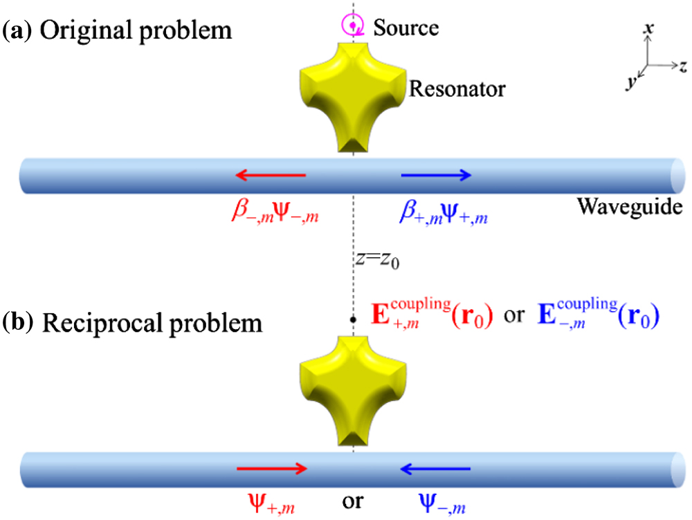
Figure 1.Schematic diagram of the indirect chiral coupling, with the resonator as a coupling interface between a point source and a waveguide. (a) Original problem under excitation by a point source at

r_{0}

, with

β_{+, m}

and

β_{-, m}

denoting the coefficients of the excited normalized

m

th waveguide modes

ψ_{+, m}

and

ψ_{-, m}

propagating in positive and negative

z

directions, respectively. (b) Reciprocal problem under excitation by the

ψ_{+, m}

and

ψ_{-, m}

with unitary coefficient, with

E_{+, m}^{coupling} (r_{0})

E_{-, m}^{coupling} (r_{0})

denoting the excited electric field at

r_{0}

, respectively. For the example of the system sketched in the figure, the source is right-handed circularly polarized (as sketched by the arrowed circle), and the structure is symmetric with respect to the

{z = z}_{0}

plane where the source is located. In the following figures, the

ψ_{+, m}

and

ψ_{-, m}

are omitted for simplicity, with only the coefficients

β_{\pm}

being labeled.

Now we consider the calculation of waveguide mode coefficients excited by a circularly polarized point source based on Eq. (1). The right-handed circularly polarized point source can be expressed as $j = j_{σ} = δ (r - r_{0}) p_{σ}$ , where $p_{σ} = x + z i$ , with $x$ and $z$ being unit vectors along the $x$ and $z$ directions, respectively. $j_{σ}$ can be decomposed into a superposition of two linearly polarized point sources $j_{x} = δ (r - r_{0}) x$ and $j_{z} = δ (r - r_{0}) z$ with orthogonal polarization directions and a phase difference of $π / 2$ , i.e., $j_{σ} = j_{x} + j_{z} i$ . In the following discussion, it is assumed that the coupling structure is symmetric with respect to the $z = z_{0}$ plane where the source is located (as sketched in Fig. 1). According to the symmetry of the electromagnetic field [73], it can be concluded that the coefficients of the $m$ th forward- and backward-propagating waveguide modes excited by $j_{x}$ are equal, which are denoted by $β_{m}^{⊥}$ ; while those excited by $j_{z}$ are opposite, which are denoted by $β_{m}^{| |}$ and $- β_{m}^{| |}$ , respectively. According to the principle of linear superposition of the electromagnetic field, $β_{+, m} = β_{m}^{⊥} + i β_{m}^{| |} = \frac{E_{x, -, m}^{coupling} (r_{0}) + i E_{z, -, m}^{coupling} (r_{0})}{⟨ ψ_{-, m} | ψ_{+, m} ⟩},$ (3a) $β_{-, m} = β_{m}^{⊥} - i β_{m}^{| |} = \frac{E_{x, +, m}^{coupling} (r_{0}) + i E_{z, +, m}^{coupling} (r_{0})}{⟨ ψ_{-, m} | ψ_{+, m} ⟩},$ (3b)where the second equalities are obtained with the use of Eq. (1), and the subscripts $x$ and $z$ denote the $x$ and $z$ components of the electric field vector $E$ . The second equalities of Eq. (3) further yield $E_{x, -, m}^{coupling} (r_{0}) = E_{x, +, m}^{coupling} (r_{0}), - E_{z, -, m}^{coupling} (r_{0}) = E_{z, +, m}^{coupling} (r_{0}) .$ (4)Note that Eq. (4) can be also consistently derived from the symmetry of the electromagnetic fields excited by the forward- and backward-propagating waveguide modes.

Next, based on Eq. (3), it is possible to explicitly demonstrate the conditions for the occurrence of chiral coupling between the circularly polarized point source and waveguide modes. Equation (3) indicates that if $E_{x, -, m}^{coupling} (r_{0}) = - i E_{z, -, m}^{coupling} (r_{0}) \Leftrightarrow E_{x, +, m}^{coupling} (r_{0}) = i E_{z, +, m}^{coupling} (r_{0}),$ (5)i.e., the T-spin of $E_{-, m}^{coupling} (r_{0})$ is consistent with the spin of $j_{σ}$ (right-handed circular polarization), or equivalently, the T-spin of $E_{+, m}^{coupling} (r_{0})$ is contrary to the spin of $j_{σ}$ , there will be $β_{+, m} = 0$ and $β_{-, m} \neq 0$ , which means the occurrence of chiral coupling that only $ψ_{-, m}$ is excited by $j_{σ}$ . Similarly, if $E_{x, +, m}^{coupling} (r_{0}) = - i E_{z, +, m}^{coupling} (r_{0}) \Leftrightarrow E_{x, -, m}^{coupling} (r_{0}) = i E_{z, -, m}^{coupling} (r_{0}),$ (6)i.e., the T-spin of $E_{+, m}^{coupling} (r_{0})$ is consistent with the spin of $j_{σ}$ , or equivalently, the T-spin of $E_{-, m}^{coupling} (r_{0})$ is contrary to the spin of $j_{σ}$ , there will be $β_{-, m} = 0$ and $β_{+, m} \neq 0$ , which means the occurrence of chiral coupling that only $ψ_{+, m}$ is excited by $j_{σ}$ .

The above analysis shows that there exists a locking effect between the propagation direction (momentum) of the waveguide mode $ψ_{\pm, m}$ and the transverse circular polarization (T-spin) of the electric field $E_{\pm, m}^{coupling} (r_{0})$ excited by $ψ_{\pm, m}$ [as shown in Eqs. (5) and (6)]. Accordingly, based on Eq. (3) derived from the reciprocity theorem, there will exist a locking effect between the circular polarization (spin) of the chiral source $j_{σ}$ and the propagation direction (momentum) of the waveguide mode excited by $j_{σ}$ .

Based on the above analysis, we will further derive some novel general relations between the directivity of the excited waveguide mode and the T-spin of the field or point source, as stated in the following.

A directivity factor $g$ of the excited waveguide mode $ψ_{\pm, m}$ can be defined as $g = (| β_{+, m} |^{2} - | β_{-, m} |^{2}) / (| β_{+, m} |^{2} + | β_{-, m} |^{2})$ , where $g = 1$ or $- 1$ means a perfect unidirectional excitation of $ψ_{+, m}$ or $ψ_{-, m}$ , respectively. The T-spin of $E_{+, m}^{coupling} (r_{0})$ can be described by the Stokes parameter [5,7,44,57], $S_{3} (r_{0}) = \frac{- 2 Im [E_{x, +, m}^{coupling} (r_{0}) E_{z, +, m}^{coupling} {(r_{0})}^{*}]}{{| E_{x, +, m}^{coupling} (r_{0}) |}^{2} + {| E_{z, +, m}^{coupling} (r_{0}) |}^{2}}$ , where $S_{3} (r_{0}) = - 1$ , 0, 1 correspond to left-handed, null, and right-handed T-spin of $E_{+, m}^{coupling} (r_{0})$ , respectively. Then from Eqs. (3) and (4), which are derived under the two assumptions that the point source is right-handed circularly polarized and that the coupling structure is symmetric with respect to the $z = z_{0}$ plane, it can be proved that the $g$ defined for the original problem and $S_{3}$ defined for the reciprocal problem satisfy a general relation (see Appendix A.2): $g = S_{3} (r_{0}) .$ (7)Equation (7) can be regarded as a generalization of Eqs. (5) and (6) for the special cases of $g = - 1$ and 1 to the general case of $- 1 \leq g \leq 1$ .

Furthermore, we consider a point source $j = δ (r - r_{0}) p$ with an arbitrary polarization, i.e., $p = p_{x} x + p_{z} z$ , and assume that the coupling structure is designed to satisfy Eq. (6), i.e., $S_{3} (r_{0}) = 1$ . Then substituting $p = p_{x} x + p_{z} z$ into Eq. (1) and using Eqs. (4) and (6), one can derive another general relation (see Appendix A.3): $g = \frac{- 2 Im (p_{x} p_{z}^{*})}{{| p_{x} |}^{2} + {| p_{z} |}^{2}} .$ (8)The right side of Eq. (8) is defined as the $S_{3}$ parameter of the point source, denoted by $S_{3, source .} S_{3, source} = - 1$ , 0, 1 correspond to left-handed circularly polarized, linearly polarized, and right-handed circularly polarized point sources, respectively, and according to Eq. (8), will lead to a unidirectional excitation of $ψ_{-, m}$ , a bidirectional excitation of both $ψ_{-, m}$ and $ψ_{+, m}$ , and a unidirectional excitation of $ψ_{+, m}$ , respectively.

Note that for Eq. (7), a change of $S_{3} (r_{0})$ or $g$ implies a change of the coupling structure while the polarization of the point source remains unchanged to be right-handed circular polarization. For Eq. (8), differently, a change of $S_{3, source}$ or $g$ implies a change of the polarization of the source while the coupling structure remains unchanged. Therefore, the significance of Eq. (7) is that it provides a general tool for designing the structure [through designing the $S_{3} (r_{0})$ ] to achieve the desired chiral coupling ( $g$ ); while the significance of Eq. (8) lies in the fact that it explicitly demonstrates the feasibility to read out the static qubit of the source ( $S_{3, source}$ ) by measuring the flying qubit of photons ( $g$ ) [1,46].

Here we emphasize that the above proposed theories are generally applicable to any direct/indirect chiral-coupling systems (i.e., waveguide without/with additional coupling structures that may support resonant modes) and to any lossless/lossy waveguide modes (i.e., propagation constants being real/complex), and can be readily extended to $z$ -periodic waveguides [72] such as the photonic crystal waveguides widely used for the chiral coupling [36 –43]. The WME-GF with a complex-conjugate form commonly used in the literature [10,11,36 –38,44,64,65] can be regarded as a special case of our theories for direct chiral-coupling systems and lossless waveguide modes. To see the point, in Appendix A.1, we provide a derivation of a general WME-GF for lossy waveguide modes based on the QNM expansion formalism [68 –71], which explicitly shows how the general WME-GF reduces to the complex-conjugate WME-GF for lossless waveguide modes. A numerical example (Fig. 8 in Appendix A.1) is provided to show the higher accuracy of the general WME-GF compared with the complex-conjugate WME-GF for lossy waveguide modes. This derivation can be regarded as an extension of the derivation of the complex-conjugate WME-GF in the literature (see Eq. (22) in Ref. [65] or Eq. (47) in Ref. [64], for instance) based on the normal-mode expansion formalism. Furthermore, the derived general WME-GF is consistent with our theories derived from the reciprocity theorem, and thus provides a logic cross-check of our theories.

Based on Eqs. (5) and (6) [or, the general relation of Eq. (7)], we then design an indirect chiral-coupling system mediated by an FP resonance of dual SPP modes on the platform of an SPP nanowire waveguide. As shown in Fig. 2(a), the system consists of three parts: a nanowire SPP waveguide, a single-wire antenna (SA), and a double-wire antenna (DA). A circularly polarized point source is located in the gap between the SA and the right terminal of the DA. The material of the structure is gold, with wavelength-dependent refractive index $n_{m}$ taking tabulated values from Ref. [74]. For the emission wavelength $λ = 750 nm$ of the source which is considered throughout this paper, there is $n_{m} = 0.1681 + 4.584 i$ . The structure is in the air environment without a substrate to simplify the analysis. All the cross sections of nanowires are square with a side length of $D = 40 nm$ . The widths of the air gap in the DA and of the gap between the SA and the right terminal of the DA are all $G = 20 nm$ . Note that high-definition ultrasmooth gold nanostructures such as nanowires with widths and gaps down to tens of nanometers are achievable experimentally [75].

Figure 2.Indirect chiral-coupling system between a chiral point source and the SPP waveguide mode mediated by an FP nanocavity. (a) Sketch of system. The circularly polarized point source (shown by the red dot) is located in the air gap between the SA and the right terminal of the DA. The coordinate origin

O

is set at the inner center of the waveguide. (b) Electric field of the fundamental SPP modes, calculated with the fully vectorial a-FMM. (b1) Distribution (in the

x − y

plane) of the electric-field modulus

| E | = \sqrt{| E_{x} |^{2} + | E_{y} |^{2} + | E_{z} |^{2}}

of the fundamental SPP mode on the waveguide and SA, which satisfies the normalization of

E_{z} = 1

at the center of the waveguide and has a complex effective index of

n_{eff} = 1.700 + 0.05136 i

. (b2) Distribution (in the

y − z

plane) of the electric-field

z

component modulus |

E_{z}

| of the fundamental antisymmetric SPP mode on the DA, which satisfies the normalization of

E_{z} = 1

at the center of the DA and has a complex effective index of

n_{eff}^{asym} = 2.423 + 0.07471 i

. (b3) Distribution of

| E_{x} |

of the fundamental symmetric SPP mode on the DA, which satisfies the normalization of

E_{x} = 1

at the center of the DA and has a complex effective index of

n_{eff}^{sym} = 1.475 + 0.03732 i

. (c) Distribution (in the plane

y = 0

) of

| E |^{2}

excited by the normalized up-going fundamental SPP on the waveguide (shown by the red arrow). The length of the DA is

L = 200 nm

and the results are obtained with the a-FMM. The superimposed dotted lines in (b) and (c) represent the boundaries of structures.

Because the size of the cross sections of the nanowires is much smaller than the wavelength, only the fundamental SPP modes of the waveguide, SA, and DA, are bounded (field decaying to null at infinity in transversal directions) and propagative (propagation constant being almost real). For the designed system, only the bounded and propagative SPP modes are needed to be considered. The reason is that with regard to the formation of the chiral field at the position of the source, the contributions of other unbounded or evanescent modes can be neglected, which can be quantitatively verified by the SPP models built up later. The waveguide and the SA only support one fundamental SPP mode, whose electric field distribution is shown in Fig. 2(b1). While the DA supports two fundamental SPP modes, whose electric-field vectors are mirror antisymmetric and symmetric with respect to $z = 0$ plane [the coordinate system shown in Fig. 2(a)], as shown in Figs. 2(b2) and 2(b3), respectively.

Figure 3.Definitions of the SPP scattering coefficients and the unknown SPP mode coefficients in the SPP model. The superscripts “sym” and “asym,” which correspond to the symmetric and antisymmetric SPPs on the DA, respectively, are omitted in the figure. (a) SPP model for the reciprocal problem. (a1) Unknown SPP mode coefficients

a_{\pm}

and

b_{\pm}

to be solved in the model. (a2)–(a4) Definitions of SPP scattering coefficients

α_{\pm}

r_{a}

, and

r_{b}

, and definition of the coupling field

ψ_{R}

. In (a1) and (a2), the blue and red arrows or coefficients correspond to the incident SPPs on the upper and lower waveguide arms, respectively. (b) SPP model for the original problem (red dot representing the point source). (b1) Unknown SPP mode coefficients

a_{s}

b_{s}

β_{+}

, and

β_{-}

to be solved in the model. (b2) Definitions of SPP excitation coefficient

γ

and field

ψ_{source}

excited by the point source. (b3) Definition of SPP coupling coefficients

χ_{\pm}

From Figs. 2(b2) and 2(b3), one can see that the antisymmetric and symmetric SPPs provide dominant electric-field components $E_{z}$ and $E_{x}$ in the gap of the DA, respectively, which are the very two field components to excite the T-spin of the field at the position of the source [see the right side of Eq. (3)]. The incident fundamental SPP mode on the waveguide will excite the antisymmetric and symmetric SPPs on the DA simultaneously. However, compared with the antisymmetric SPP, the FP resonance of the symmetric SPP on the DA is weaker because of the weaker confinement of the field, which results in a weaker $E_{x}$ than $E_{z}$ . To overcome this difficulty, we put the SA close to the right terminal of the DA. Thus, when the SA is at an FP resonance, the $E_{x}$ in the gap between the DA and the SA will be enhanced significantly, so that a chiral electric field can be constructed. Here, the length of the SA is set as $L_{SA} = 370 nm$ , making the SA at a lower order of FP resonance (for which the $L_{SA}$ is smaller and the resonance is stronger). The calculation process to determine the $L_{SA}$ is provided in Appendix B.1.

Figure 2(c) shows that for specific lengths of the DA, an incident forward-propagating SPP on the waveguide can excite the FP resonances of both the DA and the SA [the field distribution at the FP resonance of the SA is shown in Fig. 9(b) of Appendix B.1], which results in an enhanced electric field in the gap between the DA and the SA. Therefore, it is expected that if a circularly polarized source is placed in the gap between the DA and the SA [as shown by the red dot in Fig. 2(a)], an indirect chiral coupling between the source and the SPP on the waveguide is likely to be achieved. A detailed analysis will be provided in the next subsection.

B. Analysis of the Chiral Coupling based on an SPP Model for the Reciprocal Problem

For the proposed chiral-coupling system, we will build up an SPP model for the reciprocal problem in which an incident SPP waveguide mode is considered based on Eq. (3), so as to provide a quantitative analysis of the physical mechanism of the chiral coupling. The model is based on a multiple-scattering process of the fundamental SPPs on the DA, in which other non-bounded or non-propagative higher-order modes are neglected, and can provide analytical expressions of the coefficients of the SPP on the waveguide excited by a circularly polarized source. All the parameters in the model are obtained with the first-principles calculations without fitting the numerical results or experimental data, which ensures a solid electromagnetic foundation and thus a quantitative prediction of the model.

According to Eq. (3), for the calculation of the coefficients $β_{+}$ and $β_{-}$ of the forward and backward fundamental SPPs on the waveguide excited by a circularly polarized source [as shown in Fig. 2(a)], the corresponding reciprocal problems are for the calculation of the electric field at the position of the source excited by an incident backward or forward fundamental SPP on the waveguide, respectively. The incident forward/up-going SPP from the bottom of the waveguide will excite the right-going and left-going symmetric (antisymmetric) SPPs on the DA with coefficients $a_{+}^{sym}$ and $b_{+}^{sym}$ ( $a_{+}^{asym}$ and $b_{+}^{asym}$ ), respectively, as shown in Fig. 3(a1). Here all the SPPs with unitary coefficients satisfy the normalizations (on the cross sections where the SPPs begin to propagate) as specified in Fig. 2(b). To determine the SPPs’ coefficients, a set of coupled-SPP equations can be written: $a_{+}^{sym} = α_{+}^{sym} + b_{+}^{sym} u^{sym} r_{b}^{sym},$ (9a) $b_{+}^{sym} = a_{+}^{sym} u^{sym} r_{a}^{sym},$ (9b) $a_{+}^{asym} = α_{+}^{asym} + b_{+}^{asym} u^{asym} r_{b}^{asym},$ (9c) $b_{+}^{asym} = a_{+}^{asym} u^{asym} r_{a}^{asym},$ (9d)where $u^{sym} = \exp (i k_{0} n_{eff}^{sym} L)$ and $u^{asym} = \exp (i k_{0} n_{eff}^{asym} L)$ are the phase-shift factors of the symmetric and antisymmetric SPPs accumulated over the DA, respectively, with $k_{0} = 2 π / λ$ being the wavenumber in vacuum, $L$ being the length of the DA, and $n_{eff}^{sym}$ and $n_{eff}^{asym}$ being the complex effective indices of the symmetric and antisymmetric SPPs, respectively, which are obtained with a fully vectorial aperiodic Fourier modal method (a-FMM) [76,77]. $α_{+}^{sym}$ ( $α_{+}^{asym}$ ) is the coefficient of the right-going symmetric (antisymmetric) SPP on a semi-infinite DA excited by the up-going SPP on the waveguide, as shown in Fig. 3(a2). $r_{a}^{sym}$ ( $r_{a}^{asym}$ ) is the reflection coefficient of a right-going incident symmetric (antisymmetric) SPP at the right terminal of a semi-infinite DA coupled with the SA, as shown in Fig. 3(a3). $r_{b}^{sym}$ ( $r_{b}^{asym}$ ) is the reflection coefficient of a left-going incident symmetric (antisymmetric) SPP at the left terminal of a semi-infinite DA coupled with the waveguide, as shown in Fig. 3(a4). Since the symmetric and antisymmetric SPPs on the DA cannot excite each other, Eqs. (9a), (9b) and Eqs. (9c), (9d) are decoupled and can be solved independently. Here $r_{a}^{sym/asym}$ and $r_{b}^{sym/asym}$ can be calculated as the scattering matrix elements [78] with the fully vectorial a-FMM. $α_{+}^{sym/asym}$ can be calculated with the mode orthogonality theorem [73,79]: $a_{+}^{sym/asym} = \frac{⟨ ψ_{-}^{sym/asym} | ψ_{+, total} ⟩}{⟨ ψ_{-}^{sym/asym} | ψ_{+}^{sym/asym} ⟩},$ (10)where $ψ_{+, total}$ is the total electromagnetic field in the structure as shown in Fig. 3(a2) excited by the up-going SPP on the waveguide, $ψ_{+}^{sym}$ and $ψ_{+}^{asym}$ ( $ψ_{-}^{sym}$ and $ψ_{-}^{asym}$ ) are the electromagnetic field of the right-going (left-going) symmetric and antisymmetric fundamental SPP modes on the DA, respectively. $ψ_{+, total}$ and $ψ_{+ / -}^{sym/asym}$ are all calculated with the a-FMM. The definition of the bilinear function $⟨ ψ_{1} | ψ_{2} ⟩$ is given by Eq. (2), with a replacement $z d x d y \to x d y d z$ and the integral plane selected to be any cross section $x = x_{1}$ of the DA.

Figure 4.Calculation results of the indirect chiral coupling. (a1) Coupling rates

Γ_{SPP, \pm}

of up-going and down-going SPPs on the waveguide excited by a right-handed circularly polarized point source plotted as functions of the length

L

of the DA, normalized by the emission rate

Γ_{air}

of the source in air. The solid curves and the circles represent the results obtained with the SPP model for the reciprocal problem [Eq. (14)] and the fully vectorial a-FMM, respectively. The blue and red curves correspond to the up-going and down-going SPPs on the waveguide, respectively. The point source is located at

r_{0} = (D / 2 + L + 7 nm

, 0, 0). (a2), (a3) Moduli

| a^{asym} |

and

| a^{sym} |

of the coefficients of the right-going antisymmetric and symmetric SPPs on the DA excited by the up-going (or down-going) SPP on the waveguide, which are obtained with the model Eq. (11a) [or Eq. (12a)]. (b) Phase difference

φ

of the two orthogonal components of the electric field at the position of the point source. The field is excited by an incident up-going SPP on the waveguide and is obtained with the model Eq. (17). (c) Directivity factor

g

obtained with the a-FMM (circles) and the SPP model (solid curve), respectively. In (a)–(c), the green vertical dashed lines from left to right correspond to

n = 0

–6 in Eq. (16). (d) Distribution (in

y = 0

plane) of

S_{3}

of the electric field in the coupling region between the DA and the SA. The field is excited by an incident up-going SPP on the waveguide and is obtained with the model Eq. (13a). (e) Distribution (in

y = 0

plane) of the normalized electric-field intensity

{(| E | / Γ_{air})}^{2}

excited by the right-handed circularly polarized point source at

r_{0}

. The result is obtained with the FEM. In (d) and (e), the length of DA is

L = 185

, 342, 500 nm from left to right, corresponding to

n = 1

, 2, 3 in (a), respectively.

Equation (9) can be understood intuitively. For Eqs. (9a) and (9c), the coefficient $a_{+}^{sym/asym}$ of the right-going SPP on the DA results from two contributions: the first one ( $α_{+}^{sym/asym}$ ) is from the direct coupling of the up-going SPP on the waveguide; the second one is from the reflection ( $r_{b}^{sym/asym}$ ) of the damped ( $u^{sym/asym}$ ) left-going SPP (with coefficient $b_{+}^{sym/asym}$ ) at the left terminal of the DA coupled with the waveguide. Equations (9b) and (9d) can be understood in a similar way. Solving Eq. (9), one can obtain $a_{+} = \frac{α_{+}}{1 - u^{2} r_{a} r_{b}},$ (11a) $b_{+} = \frac{α_{+} u r_{a}}{1 - u^{2} r_{a} r_{b}},$ (11b)where the superscripts “sym” and “asym” are omitted since $a_{+}^{sym}$ and $a_{+}^{asym}$ ( $b_{+}^{sym}$ and $b_{+}^{asym}$ ) have exactly the same form of expression. For the case of an incident backward/down-going SPP from the top of the waveguide, the coefficients of the excited right-going and left-going symmetric (antisymmetric) SPPs on the DA are denoted by $a_{-}^{sym}$ and $b_{-}^{sym}$ ( $a_{-}^{asym}$ and $b_{-}^{asym}$ ), respectively, as shown in Fig. 3(a1). The coefficient of the right-going symmetric (antisymmetric) SPP on the semi-infinite DA excited by the down-going SPP on the waveguide is denoted by $α_{-}^{sym}$ ( $α_{-}^{asym}$ ), as shown in Fig. 3(a2). Fully parallel to Eq. (11), through building up an SPP model, one can obtain $a_{-} = \frac{α_{-}}{1 - u^{2} r_{a} r_{b}},$ (12a) $b_{-} = \frac{α_{-} u r_{a}}{1 - u^{2} r_{a} r_{b}},$ (12b)where the superscripts “sym” and “asym” are omitted as well.

The electromagnetic field in the coupling region between the SA and the right terminal of the DA excited by an incident up-going or down-going SPP on the waveguide can be respectively expressed as $ψ_{+}^{coupling} (r) = a_{+}^{sym} u^{sym} ψ_{R}^{sym} (r) + a_{+}^{asym} u^{asym} ψ_{R}^{asym} (r),$ (13a) $ψ_{-}^{coupling} (r) = a_{-}^{sym} u^{sym} ψ_{R}^{sym} (r) + a_{-}^{asym} u^{asym} ψ_{R}^{asym} (r),$ (13b)where $ψ_{R}^{sym}$ ( $ψ_{R}^{asym}$ ) represents the field in the coupling region excited by the right-going symmetric (antisymmetric) SPP on the DA with unitary coefficient [as shown in Fig. 3(a3)], and can be calculated with the fully vectorial a-FMM. To achieve the chiral coupling, a circularly polarized point source is placed in the gap between the DA and the SA, with coordinate $r_{0} = (D / 2 + L + Δ x, 0, 0)$ and $Δ x$ to be determined hereafter [see the coordinate in Fig. 2(a)]. Substituting Eq. (13) into Eq. (3), one can obtain the coefficients of the up-going and down-going SPPs excited by the circularly polarized point source: $β_{+} = \frac{a_{-}^{sym} u^{sym} E_{x, R}^{sym} (r_{0}) + i a_{-}^{asym} u^{asym} E_{z, R}^{asym} (r_{0})}{⟨ ψ_{-} | ψ_{+} ⟩},$ (14a) $β_{-} = \frac{a_{+}^{sym} u^{sym} E_{x, R}^{sym} (r_{0}) + i a_{+}^{asym} u^{asym} E_{z, R}^{asym} (r_{0})}{⟨ ψ_{-} | ψ_{+} ⟩},$ (14b)where $ψ_{+}$ and $ψ_{-}$ represent the up-going and down-going fundamental SPP modes on the waveguide, respectively, $E_{x, R}^{sym}$ is the $x$ component of the electric field of $ψ_{R}^{sym}$ , and $E_{z, R}^{asym}$ is the $z$ component of the electric field of $ψ_{R}^{asym}$ . In Eq. (14), the symmetry of the structure with respect to the $z = 0$ plane yields $a_{+}^{sym} = a_{-}^{sym} = a^{sym}, a_{+}^{asym} = - a_{-}^{asym} = a^{asym},$ (15)which is consistent with Eq. (4). Equation (14) indicates that the two SPPs with different symmetries on the DA provide two regulable coefficients $a^{sym} u^{sym}$ and $a^{a sym} u^{a sym}$ for the two orthogonal electric-field components $E_{x, R}^{sym} (r_{0})$ and $E_{z, R}^{asym} (r_{0})$ that constitute the T-spin, respectively. Specifically, Eqs. (11a) and (12a) show that $a^{sym} u^{sym}$ and $a^{a sym} u^{a sym}$ can be regulated by changing the length $L$ of the DA [via the phase shift factor $u^{sym/asym} = \exp (i k_{0} n_{eff}^{sym/asym} L)$ ], which allows the possibility to form a T-spin field for an incident SPP, or reciprocally, the chiral coupling of the SPP, as to be shown in Fig. 4.

After obtaining $β_{\pm}$ , one can then calculate $Γ_{SPP, +}$ and $Γ_{SPP, -}$ , the coupling rates of the up-going and down-going SPPs on the waveguide excited by the point source, which are expressed as $Γ_{SPP, \pm} = | β_{\pm} |^{2} \iint_{z = z_{0}} \frac{1}{2} Re (E_{\pm} \times H_{\pm}^{*}) \cdot (\pm z) d x d y$ , with $z = z_{0}$ being the cross section of the waveguide where the SPP begins to propagate. The curves of $Γ_{SPP, \pm}$ as functions of the length $L$ of the DA are shown in Fig. 4(a1), with $Γ_{SPP, \pm}$ normalized by $Γ_{air}$ , the spontaneous emission rate of the circularly polarized point source $j_{σ}$ in air. $Γ_{air} = η_{vac} k_{0}^{2} n_{a} / (6 π)$ with $η_{vac}$ being the wave impedance in vacuum, and $n_{a} = 1$ being the refractive index of air. In the calculation, the source is located at $r_{0} = (D / 2 + L + 7 nm, 0, 0)$ . Note that a localization accuracy of a single quantum-dot emitter better than 2 nm has been achieved experimentally [80]. In Fig. 4(a), the results obtained with the fully vectorial a-FMM and SPP model [Eq. (14)] are shown with circles and solid curves, respectively. Good agreement can be observed between the two results, which confirms the validity of the model. Here the calculation of the $β_{\pm}$ with the a-FMM is the same as Eq. (10): the total field excited by the source is calculated with the a-FMM first, and then the $β_{\pm}$ are extracted from the total field with the mode orthogonality theorem [73,79].

Figure 4(a1) shows that for some specific values of $L$ (at the green vertical dashed lines of $n = 0$ , 1, 3 in the figure), one of $Γ_{SPP, +}$ and $Γ_{SPP, -}$ reaches the peak value and obtains significant enhancement ( $Γ_{SPP, \pm} / Γ_{air} ≫ 1$ ), while the other is almost zero. This means the occurrence of perfect chiral coupling of the SPP waveguide mode, and the corresponding $L$ are called perfect chiral points (PCPs) here. In addition, without changing the chirality of the source, the unidirectional excitation of the SPP on the waveguide can be reversed in direction (between $n = 0$ , 1 and $n = 3$ ) or disappear (at $n = 2$ ) simply by changing $L$ . The $L$ corresponding to the latter are called perfect non-chiral points (PNCPs). At the PCPs of $n = 0$ , 1, 3, the footprints of the coupling structure are $L + G + D = 102$ , 245, 560 nm in the $x$ direction, respectively, and are all $L_{SA} = 370 nm$ in the $z$ direction, which are much smaller than the footprints (from several to more than 100 μm) of the dielectric whispering-gallery microcavities with chiral-coupling structures [32,34,50,63].

To explain the above numerical phenomena, Figs. 4(a2) and 4(a3) respectively show the moduli of the coefficients of the antisymmetric and symmetric SPPs on the DA, $| a^{asym} |$ and $| a^{sym} |$ , which are given by model Eq. (11a) or (12a). The results reveal that the PCPs and PNCPs shown in Fig. 4(a1) almost exactly correspond to the different orders of FP resonance of the antisymmetric SPP on the DA, which are achieved under the phase-matching condition, $2 k_{0} Re (n_{neff}^{asym}) L + \arg (r_{a}^{asym}) + \arg (r_{b}^{asym}) = 2 n π .$ (16)Equation (16) is obtained by minimizing the denominator in Eq. (11a) or (12a) for $a^{asym}$ , and resultantly, maximizing $| a^{asym} |$ [see Fig. 4(a2)]. In Eq. (16), Re(·) denotes the real part, arg(·) denotes the argument, and $n$ is an integer corresponding to different orders of resonance [shown by the green vertical dashed lines in Figs. 4(a)–4(c)]. Equation (16) can be understood intuitively as follows: the phase change accumulated by the antisymmetric SPP that propagates back and forth over one round on the DA is multiples of $2 π$ , which obviously results in a constructive interference of the multiple-scattered SPPs and thus forms the FP resonance.

To analyze the impact of the FP resonance on the chirality of the electric field at the position of the source, Eq. (13) gives that the two orthogonal components of the electric field excited by the incident SPP on the waveguide are $E_{x, +}^{coupling} (r_{0}) = E_{x, -}^{coupling} (r_{0}) = E_{x}^{coupling} (r_{0}) = a^{sym} u^{sym} E_{x, R}^{sym} (r_{0}),$ (17a) $E_{z, +}^{coupling} (r_{0}) = - E_{z, -}^{coupling} (r_{0}) = E_{z}^{coupling} (r_{0}) = a^{asym} u^{asym} E_{z, R}^{asym} (r_{0}) .$ (17b)For the symmetric SPP on the DA, Fig. 4(a3) shows that the value of $| a^{sym} |$ is smaller with a weak fluctuation compared to $| a^{asym} |$ at resonance as the length $L$ of the DA varies, which implies a weaker FP resonance of the symmetric SPP than that of the antisymmetric SPP. However, since the SA at a specific FP resonance is placed near the right terminal of the DA, the value of $| E_{x, R}^{sym} (r_{0}) |$ is larger than that of $| E_{z, R}^{asym} (r_{0}) |$ [ $E_{x, R}^{sym} (r_{0}) = 3.9838 - 11.358 i$ and $E_{z, R}^{asym} (r_{0}) = 1.3206 - 5.3317 i$ ], which thus compensates for the smaller value of $| a^{sym} |$ than that of $| a^{asym} |$ at resonance, so that the relation $| E_{x}^{coupling} (r_{0}) | \approx | E_{z}^{coupling} (r_{0}) |$ can be achieved under the phase-matching condition of Eq. (16). The above analysis confirms the expectation of using the DA and SA to respectively enhance the $E_{z}$ and $E_{x}$ components at the source position in the gap between the DA and the SA as stated in Section 3.A.

Next, we check the phase difference $φ = \arg [E_{z}^{coupling} (r_{0}) / E_{x}^{coupling} (r_{0})]$ of the two orthogonal components of the electric field at the position of the source under the phase-matching condition. Figure 4(b) shows the $φ$ as a function of $L$ for an incident up-going SPP on the waveguide. Corresponding to $n = 0$ , 1, 2, 3 in Eq. (16), there are $φ \approx π / 2$ , $π / 2$ , 0, $- π / 2$ , i.e., the right-handed, right-handed, null, and left-handed T-spins of the electric field are excited at $r_{0}$ , respectively. Accordingly, for the original problem, if a right-handed circularly polarized source is placed at $r_{0}$ with $L$ taking values corresponding to $n = 0$ , 1, 2, 3 in Eq. (16), the forward, forward, bidirectional, and backward SPP will be launched on the waveguide, respectively.

To quantitatively describe the directional excitation of the up-going or down-going SPP on the waveguide by the chiral source, Fig. 4(c) shows the dependence of the directivity factor $g$ on $L$ . For the $L$ given by Eq. (16) with $n = 0$ , 1, 2, 3, there are $g = 0.842$ , 0.999, 0.0510, $- 0.892$ , respectively. In addition, $g$ can take values continuously over almost the whole range of [−1, 1] simply by changing $L$ (instead of changing the chirality of the source [29,37,44 –46,48] or putting the source on the other side of the waveguide [57,59]), which provides flexible freedoms for the design of chiral-coupling devices. Note that the poorer negative value of $g = - 0.892$ at $n = 3$ than the positive value of $g = 0.999$ at $n = 1$ can be further improved by adjusting the excitation and structural parameters with the aid of Eq. (7) and the SPP model. For instance, if the point source is moved from $r_{0} = (D / 2 + L + 7 nm, 0, 0)$ to $r_{0} = (D / 2 + L + 5 nm, 0, 0)$ , $g$ at $n = 3$ can be improved to be −0.964, with a moderate decrease of $g$ at $n = 1$ to 0.959.

Next we will provide a direct numerical observation for the formation of the chiral/non-chiral light field in the reciprocal problem, and for the unidirectional/bidirectional excitation of the SPP on the waveguide in the original problem, as predicted by the SPP model above. For the reciprocal problem, we calculate the spatial distribution of the Stokes parameter $S_{3}$ defined before Eq. (7) under the excitation of an up-going SPP on the waveguide. The results are obtained with the model [Eq. (13a)] and are shown in Fig. 4(d). It can be seen that for $L = 185$ , 342, 500 nm (corresponding to $n = 1$ , 2, 3), right-handed circularly polarized, linearly polarized, and left-handed circularly polarized electric fields at $r_{0}$ [corresponding to $S_{3} (r_{0}) = 0.999$ , 0.0151, −0.897] are excited by the up-going SPP on the waveguide, respectively. For the original problem, a right-handed circularly polarized source is placed at $r_{0}$ and $L$ also takes the above three values. The distributions of the excited electric field are calculated with the finite element method (FEM) executed with the software of COMSOL Multiphysics. As shown in Fig. 4(e), the results manifest that for these three values of $L$ , forward, bidirectional, and backward SPPs (corresponding to $g = 0.999$ , 0.0510, −0.892 obtained with the a-FMM) are excited on the waveguide, respectively. These results confirm the prediction of the SPP model and also the validity of the general relation Eq. (7) [note that the slight difference between $S_{3} (r_{0})$ and $g$ is due to the slight error of the SPP model relative to the a-FMM calculation].

In addition, Fig. 4(e) shows that the SA is excited to the designed FP resonance [see Fig. 9(b) in Appendix B.1], which enhances the electric-field component $E_{x}$ in the gap between the DA and the SA, and thus meets the requirement for a chiral coupling as described in a previous subsection. Meanwhile, one can observe a standing wave formed by the two counter-propagating antisymmetric SPPs on the DA at FP resonance, and the number of nodes of field increases with the increase of $L$ .

The general relation of Eq. (8) predicts that if the coupling structure is designed to satisfy $S_{3} (r_{0}) = 1$ (i.e., to achieve a perfect chiral coupling), the polarization of the excitation source ( $S_{3, source}$ ) will be directly related to the directivity of the excited SPP ( $g$ ), thus demonstrating the feasibility to read out the static qubit of the source ( $S_{3, source}$ ) by measuring the flying qubit of photons ( $g$ ) [1,46]. To confirm this prediction, we fix the structure with $L = 185 nm$ [corresponding to $n = 1$ in Eq. (16)], for which there is $S_{3} (r_{0}) = 0.999$ , and check the excitation of the SPP waveguide mode by a point source of various polarizations. Figure 4(e) with $n = 1$ and Fig. 5(a) show that the direction of the excited SPP will be reversed if the source is changed from right-handed to left-handed circular polarization. Figures 5(b)–5(d) show that the excitation of the SPP becomes bidirectional if the source is of linear or elliptical polarization. More specifically, there are $Γ_{SPP, +} / Γ_{air} (Γ_{SPP, -} / Γ_{air}) = 40.36 (0.01268), 0.01268 (40.36), 20.46 (20.46), 30.51 (10.33), 10.33 (30.51)$ , and $g = 0.999$ , −0.999, 0.00768, 0.494, −0.494 (obtained with the a-FMM) for Fig. 4(e) with $n = 1$ and Figs. 5(a)–5(d), for which $S_{3, source} = 1$ , −1, 0, 0.5, −0.5, respectively. Therefore, the prediction of the general relation Eq. (8) is confirmed. Note that the slight difference between $g$ and $S_{3, source}$ is due to the slight error of $S_{3} (r_{0})$ relative to 1.

Figure 5.Distribution (in

y = 0

plane) of the normalized electric-field intensity

(| E | / Γ_{air})^{2}

excited by a point source at

r_{0}

which is (a) left-handed circularly polarized, (b) linearly polarized in direction of 45° from the

x

axis, (c) right-handed elliptically polarized [

p = x (\sqrt{3} - 1) / 2 + i z (\sqrt{3} + 1) / 2

], or (d) left-handed elliptically polarized [

p = x (\sqrt{3} - 1) / 2 - i z (\sqrt{3} + 1) / 2

]. In (a)–(d), the length of DA is

L = 185 nm

, corresponding to

n = 1

in Eq. (16). The results are obtained with the FEM.

C. Analysis of the Purcell Factor and Chiral-Coupling Efficiency Based on an SPP Model for the Original Problem

The enhancement of the spontaneous emission rate is described by $F_{P} = Γ_{total} / Γ_{air}$ , called the Purcell factor [81,82], where $Γ_{total}$ is the total spontaneous emission rate (proportional to emission power) of the source in the designed structure. A high value of $F_{P}$ is important for the realization of an on-chip ultrafast emission source [83]. For the chiral-coupling system studied in this paper, higher $F_{P}$ means a faster readout of spin qubits from the source, that is, a higher conversion rate from the static qubits of matter to the flying qubits of photons [66]. For a right-handed circularly polarized electric dipole source $j_{σ} = (x + z i) δ (r - r_{0})$ , there is $Γ_{total} = - {Re [E_{x} (r_{0})] + Im [E_{z} (r_{0})]} / 2$ , where $E_{x} (r_{0})$ and $E_{z} (r_{0})$ are respectively the $x$ and $z$ components of the electric field excited by the source at $r_{0}$ .

The coupling efficiency of the SPP on the waveguide excited by the source is defined as $η_{\pm} = Γ_{SPP, \pm} / Γ_{total}$ [1,64,66,81], which describes the probability for emitted photons to be channeled into the up-going or down-going SPP waveguide mode [66]. Improvement of $η_{\pm}$ is of great significance for improving the signal intensity of the waveguide mode in the on-chip single photon source and integrated photonic circuits [1,37].

To analyze the $F_{P}$ and $η_{\pm}$ , an SPP model can be built up as well for the original problem [as illustrated in Fig. 3(b) and detailed in Appendix B.2]. With the model [Eq. (B3) in Appendix B.2], the total spontaneous emission rate can be expressed as $Γ_{total} = - \frac{1}{2} Re [E_{x, source} (r_{0}) + a_{s}^{sym} u^{sym} E_{x, R}^{sym} (r_{0})] - \frac{1}{2} Im [E_{z, source} (r_{0}) + a_{s}^{asym} u^{asym} E_{z, R}^{asym} (r_{0})] .$ (18)Equation (18) shows that the two SPPs with different symmetries on the DA provide two regulable coefficients $a_{s}^{sym} u^{sym}$ and $a_{s}^{asym} u^{asym}$ for $Γ_{total}$ , which depend on the length $L$ of the DA [via the phase shift factor $u$ ; see Eq. (B2a) in Appendix B.2].

In addition, with the SPP model for the original problem, analytical expression of the coefficient $β_{\pm}$ of the SPP waveguide mode excited by the source can be obtained as well; see Eq. (B4) in Appendix B.2. As expected, with the reciprocity theorem [72,73] it can be proved that the $β_{\pm}$ given by the SPP models for the original problem and the reciprocal problem [see Eq. (14)] are identical, as shown in Appendix B.2.

The dependence of the Purcell factor $F_{P}$ on the length $L$ of the DA is shown in Fig. 6(a). The results obtained with the SPP model [Eq. (18)] are in good agreement with the rigorous numerical results of the a-FMM, which confirms the validity of the model. At the PCPs and PNCPs ( $n = 0$ , 1, 2, 3) shown in Fig. 4(a1), $F_{P}$ reaches high peak values of 119, 203, 152, and 145, respectively, exhibiting a significant enhancement of the spontaneous emission rate of the chiral source. These high peak values of $F_{P}$ result from the fact that under the phase-matching condition of Eq. (16), the coefficient $a_{s}^{asym}$ of the antisymmetric SPP in Eq. (18) will take a maximum value.

Figure 6.Purcell factor

F_{P} = Γ_{total} / Γ_{air}

of the chiral source and coupling efficiency

η_{\pm}

of the SPP waveguide mode. The solid curves and the circles represent the results obtained with the SPP model for the original problem and the fully vectorial a-FMM, respectively. The green vertical dashed lines from left to right correspond to

n = 0

–6 in Eq. (16). (a) Results of the Purcell factor

Γ_{total} / Γ_{air}

of a chiral point source of right-handed circular polarization at

r_{0} = (D / 2 + L + 7 nm

, 0, 0). (b) Results of the coupling efficiency

η_{\pm} = Γ_{SPP, \pm} / Γ_{total}

of the up-going (blue curve) and down-going (red curve) SPPs on the waveguide excited by the chiral point source at

r_{0}

Figure 7.Integral path (blue lines) and poles (red dots) of the integrand for the integration in Eq. (A8). (a) and (b) are for the cases of

z - z_{0} > 0

and

z - z_{0} < 0

, respectively. For

z - z_{0} > 0

(

z - z_{0} < 0

), the closed integral path is composed of the real axis and a semi-circle

C_{+}

(

C_{-}

) in the upper (lower) complex plane with an infinite radius

R

, in which the integrand

f (k)

has a single first-order pole of

k_{m}

(

- k_{m}

Figure 8.Numerical example showing the higher accuracy of Eq. (A17) (our theory) compared with Eq. (A19) (previous theories) for lossy waveguide modes. (a) Sketch of the direct chiral-coupling system composed of a gold-nanowire waveguide and a nearby chiral source (the red dot). The waveguide is identical to that considered in Fig. 2(b1) in the main text and supports the fundamental lossy SPP mode as shown in Fig. 2(b1). A right-handed circularly polarized point source is located at

r_{0} = (x_{0}, y_{0}, z_{0}) = (D / 2 + 15 nm, 0, 0)

, with the coordinate origin

O

set at the inner center of the waveguide. (b) Relative error of

E_{z, +} (0)

of the excited forward-propagating SPP waveguide mode (see its detailed definition in the text) obtained with Eq. (A17) (blue solid curve) and Eq. (A19) (blue dashed curve) for different wavelengths. The inset shows the imaginary part of the complex effective index

n_{eff}

of the SPP waveguide mode plotted as a function of the wavelength. In calculating the

E_{z, +} (0)

with Eq. (A17), Eq. (A19), and the mode-orthogonality theorem, the full-wave aperiodic Fourier modal method (a-FMM) [74,75] is used to obtain the fundamental SPP waveguide mode and the total electromagnetic field excited by the point source.

The results of the coupling efficiency $η_{\pm}$ of the SPP on the waveguide are shown in Fig. 6(b). At the PCPs and PNCPs ( $n = 0$ , 1, 2, 3), there are $η_{+} = 44 %$ ( $η_{-} = 4.7 %$ ), 25% (0.028%), 10% (10%), and 0.87% (16%), respectively, exhibiting an efficient unidirectional or bidirectional coupling of the SPP. The values of $η_{\pm}$ could be further improved by optimizing the system parameters with the aid of the SPP model, for instance, to suppress the SPP propagation loss [84] or non-radiative decay rate [81,85] by optimizing the sizes and materials of the DA and the SA and their in-between gaps.

D. Comparative Discussions on the Performance of the Indirect Chiral-Coupling System

As shown in Appendix B.3, the system without the SA exhibits a weaker unidirectionality of the excited SPP waveguide mode [Figs. 10(a1) and 10(b1)]. For a bare SPP waveguide (acting as a direct chiral-coupling system [57,59]) in comparison with the proposed indirect chiral-coupling system, the former exhibits obviously poorer performances, regarding the effective-coupling distance, the directivity factor $g$ , the coupling efficiency $η_{\pm}$ of the SPP waveguide mode, and the Purcell factor $F_{P}$ of the chiral source [Figs. 10(a2), 10(b2), and 11]. These comparative results show the performance advantages of the proposed indirect chiral-coupling system.

Figure 9.(a) Total spontaneous emission rate

Γ_{total}

of an

x

-polarized point source plotted as a function of the length

L_{SA}

of the SA.

Γ_{total}

is normalized by the spontaneous emission rate

Γ_{air}

of the point source in air, with

Γ_{air}

η_{vac} k_{0}^{2} n_{a} / (12 π)

. The structure and coordinate system are shown in the inset, with coordinate origin

O

at the inner center of the antenna. The coordinate of the point source (shown by the red dot) is

(x, y, z) = (- D / 2 - 13 nm, 0, 0)

, with

D = 40 nm

being the side length of the antenna cross section. (b) Distribution of normalized electric-field intensity

(| E | / Γ_{air})^{2}

excited by the point source, obtained for

L_{SA} = 370 nm

and in sections

y = 0

(left) and

x = 0

(right).

Figure 10.Distribution (in

y = 0

plane) of the normalized electric-field intensity

(| E | / Γ_{air})^{2}

in the structure without the SA (a1) or without the DA and the SA (a2), which is excited by a right-handed circularly polarized point source at

r_{0}

corresponding to a DA length of

L = 185 nm

[i.e.,

n = 1

in Eq. (16)]. (b1), (b2) The same as (a1) and (a2) but for

L = 500 nm

[i.e.,

n = 3

in Eq. (16)]. The results are obtained with the FEM.

Figure 11.(a) Sketch of the direct chiral-coupling system, which is composed of a bare SPP waveguide excited by a nearby right-handed circularly polarized point source (shown by the red dot). The waveguide is a gold nanowire with a square cross section of side length

D = 40 nm

(identical to the waveguide in the indirect chiral-coupling system proposed in the main text). The point source is located at

r_{0} = (D / 2 + d, 0, 0)

, with the coordinate origin

O

set at the inner center of the waveguide. (b) Purcell factor

F_{P} = Γ_{total} / Γ_{air}

of the point source plotted as a function of the source-waveguide distance

d

. (c) Coupling efficiency

η_{\pm} = Γ_{SPP, \pm} / Γ_{total}

of the up-going (blue curve) and down-going (red curve) fundamental SPP modes on the waveguide, and the directivity factor

g

(green curve) plotted as functions of

d

. The results are obtained with the full-wave a-FMM.

As shown in Appendix B.4 (Fig. 12), the performances of the proposed indirect chiral-coupling system can be largely preserved after adding a substrate and considering the actual location of a quantum-dot emitter on the substrate [37,39,44 –46,48,64]. This exhibits the robustness of performances and feasibility of an experimental demonstration for the proposed indirect chiral-coupling system with practical configurations.

Figure 12.(a) Sketch of the indirect chiral-coupling system on a glass substrate in air. The gold nanowires have a square cross section with a side length

D = 40 nm

, and the gaps in the DA and between the DA and SA are all of width

G = 20 nm

, which are identical to those of the system without a substrate. The coordinate origin

O

is set at the inner center of the waveguide. The right-handed circularly polarized point source is located at

r_{0} = (D / 2 + L + 7 nm

, 15 nm, 0), with

L

being the length of the DA. The length of the SA is

L_{SA} = 290 nm

. (b) Coupling rates

Γ_{SPP, \pm}

of up-going (blue curve) and down-going (red curve) fundamental SPP modes on the waveguide excited by the point source, which are plotted as functions of

L

and normalized by the emission rate

Γ_{air}

of the source in air. (c) Directivity factor

g

of the excited SPPs. (d) Purcell factor

F_{P} = Γ_{total} / Γ_{air}

of the point source. (e) Coupling efficiency

η_{\pm} = Γ_{SPP, \pm} / Γ_{total}

of the up-going (blue curve) and down-going (red curve) SPPs. In (b)–(e), the results are obtained with the full-wave FEM. The vertical green-dashed lines show the values of

L

determined by the phase-matching condition of Eq. (16) in the main text.

We propose a general approach based on the reciprocity theorem for an intuitive analysis and rigorous calculation of the coupling coefficient between the chiral source and the waveguide mode. With this approach, we derive the conditions for the occurrence of chiral coupling as well as some general relations between the chiral-coupling directivity ( $g$ ) and T-spin ( $S_{3}$ ) of the field or source.

Based on the theories, a novel indirect chiral-coupling system between a chiral emitter and waveguide modes mediated by FP resonance is proposed, which is on the platform of SPP with a deep subwavelength scale. Compared with the direct chiral-coupling system, this system gets rid of the restriction that the emission source must be in the limited evanescent-field region of the waveguide mode. As a mediator, the FP resonance provides flexible freedoms to regulate the chiral coupling, and can achieve nearly perfect chiral coupling, non-chiral coupling, and a direction reversal of the chiral coupling without changing the chirality of the source. In addition, with the assistance of the FP resonance, high spontaneous-emission-enhancement Purcell factor of the chiral source and high chiral-coupling efficiency between the source and the SPP waveguide mode are obtained, which enables the system to realize a deterministic, fast, and efficient readout of the spin qubits in the source. The proposed chiral-coupling system is expected to be realizable in experiment in view of the current fabrication and testing capabilities [77,80] and our simulation results for practical configurations.

To explore the underlying physical mechanism of the indirect chiral-coupling system, two SPP models based on first principles are built up by considering the excitation and multiple scattering processes of SPPs in the structure. The SPP model for the reciprocal problem indicates that the T-spin at the position of the source originates from two SPPs with different symmetries supported by the structure, and that an emergence, disappearance, and flip of T-spin can be realized simply by adjusting the antisymmetric SPP to reach different orders of FP resonance. The SPP model for the original problem clarifies that once the antisymmetric SPP is at an FP resonance, the spontaneous-emission-enhancement Purcell factor will reach the maximum, and the chiral-coupling efficiency between the source and the SPP waveguide mode will take a large value.

We expect that our proposed theories will provide general recipes for an intuitive and quantitative design of various direct/indirect chiral-coupling systems. Thanks to the FP resonance with flexible design freedoms and rich implementation platforms (such as SPP platforms [79,86] and photonic-mode dielectric platforms [87,88]), indirect chiral-coupling systems with the FP resonance as coupling intermediaries can be further developed based on the work of this paper to achieve improved performances and extended applications.

APPENDIX A: SOME GENERAL THEORETICAL DERIVATIONS ABOUT THE CHIRAL COUPLING OF AN EMITTER TO WAVEGUIDE MODES

In this section, we will provide a derivation of a general WME-GF for lossy waveguide modes based on the QNM expansion formalism [68–71]. This derivation will explicitly show how the general WME-GF reduces to the complex-conjugate WME-GF commonly used in the literature [10,11,36–38,44,64,65] for lossless waveguide modes, as mentioned in the main text (the end of Section 2). Finally, we will provide a numerical example showing the higher accuracy of the general WME-GF compared with the complex-conjugate WME-GF for lossy waveguide modes.

The QNM is a rigorous conceptualization of the resonant mode commonly referred to in the literature. It is the eigensolution of the source-free Maxwell’s equations and satisfies the outgoing-wave condition at infinity [68–71]. It corresponds to a complex-valued eigenfrequency for generally lossy systems and reduces to the normal mode (NM) with a real-valued eigenfrequency for lossless systems [69]. Therefore, our derivation here can be regarded as an extension of the derivation of the complex-conjugate WME-GF based on the NM expansion (see Eq. (22) in Ref. [65] or Eq. (47) in Ref. [64], for instance).

To obtain the Green’s function of a waveguide, we consider a point source expressed as an electric current density

j = p δ (x - x_{0}) δ (y - y_{0}) δ (z - z_{0})

located at the vicinity of the waveguide, with the

z

axis set along the translationally invariant direction of the waveguide [as illustrated by Fig. 1(a) in the main text with the resonator removed]. With the Fourier expansion of the Dirac

δ

-function,

δ (z - z_{0}) = \frac{1}{2 π} \int_{- \infty}^{+ \infty} \exp [i k (z - z_{0})] d k,

(A1)

the point source can be expressed as

j (r) = \frac{1}{2 π} \int_{- \infty}^{+ \infty} p δ (x - x_{0}) δ (y - y_{0}) \exp [i k (z - z_{0})] d k .

(A2)

Equation (A2) shows that the point source

j

an be expressed as a superposition of infinite number of line current sources

j^{'} (r, k) = \frac{1}{2 π} p δ (x - x_{0}) δ (y - y_{0}) \exp [i k (z - z_{0})]

, which is located at (

x_{0}

y_{0}

) and has a definite wave vector

k

along the

z

direction.

In the following, we will apply the QNM expansion formalism to obtain the electric field

E^{'}

excited by

j^{'}

, and a superposition of

E^{'}

with various

k

then gives the electric field

E

excited by

j

. For this purpose, the electric field of the

m

th QNM with the wave vector

k

on the waveguide can be expressed as

E_{m} (r, k) = E_{m} (ρ, k) \exp (i k z),

(A3)

where

r = (x, y, z)

and

ρ = (x, y, 0)

. According to the QNM-expansion formalism [68–71] for a waveguide of generally lossy and dispersive reciprocal materials,

E^{'}

excited by

j^{'}

can be expanded onto the basis of the QNMs as

E^{'} (r, r_{0}, k) = \sum_{m = 1}^{\infty} C_{m} (r_{0}, k) E_{m} (ρ, k) \exp (i k z),

(A4)

where the expansion coefficients are expressed as

C_{m} (r_{0}, k) = \frac{p \cdot E_{m} (ρ_{0}, - k) \exp (- i k z_{0})}{2 π i [ω - ω_{m} (k)] P_{m} (k)},

(A5)

with

r_{0} = (x_{0}, y_{0}, z_{0})

ρ_{0} = (x_{0}, y_{0}, 0)

ω

denoting the real-valued excitation angular frequency,

ω_{m} (k)

denoting the complex-valued eigenfrequency of the QNM, and a pseudoenergy of the QNM expressed as

P_{m} (k) = \iint_{- \infty}^{+ \infty} d x d y {E_{m} (ρ, k) \cdot \frac{\partial [ω ε (ω)]}{\partial ω} |_{ω = ω_{m}} \cdot E_{m} (ρ, - k) - H_{m} (ρ, k) \cdot \frac{\partial [ω μ (ω)]}{\partial ω} |_{ω = ω_{m}} \cdot H_{m} (ρ, - k)} .

(A6)

In Eq. (A6),

ε

and

μ

represent the permittivity and permeability tensors of the waveguide material, respectively, and satisfy

ε^{T} = ε

and

μ^{T} = μ

for reciprocal materials. According to Eq. (A2), the electric field excited by

j

is then expressed as

E (r, r_{0}) = \int_{- \infty}^{+ \infty} E^{'} (r, r_{0}, k) d k .

(A7)

Substituting Eq. (A5) into Eq. (A4) and then into Eq. (A7), one can obtain

E (r, r_{0}) = \sum_{m = 1}^{\infty} \int_{- \infty}^{+ \infty} f (k) d k,

(A8)

with

f (k) = \frac{\exp [i k (z - z_{0})]}{2 π i [ω - ω_{m} (k)] P_{m} (k)} p \cdot E_{m} (ρ_{0}, - k) E_{m} (ρ, k) .

(A9)

Now we consider the calculation of the integral

\int_{- \infty}^{+ \infty} f (k) d k

in Eq. (A8), which will be performed with the residue theorem [89]. For this purpose, we first analyze the poles of the integrand

f (k)

in the complex plane of

k

. Equation (A9) of

f (k)

shows that

f (k)

has first-order complex poles satisfying

ω = ω_{m} (k)

, which can be equivalently expressed as

k = \pm k_{m} (ω)

with

Re (k_{m}) > 0

and

Im (k_{m}) > 0

, as shown with the red dots in Fig. 7. Here the

k = \pm k_{m} (ω)

are nothing else than the dispersion relations of the propagation constants of the

m

th forward (+) and backward (−) traveling waveguide modes for a given real-valued excitation frequency

ω

For the case of

z - z_{0} > 0

, we construct a closed integral path as shown in Fig. 7(a), and calculate the integral

\int_{- \infty}^{+ \infty} f (k) d k

\int_{- \infty}^{+ \infty} f (k) d k = \int_{- \infty}^{+ \infty} f (k) d k + \int_{C^{+}} f (k) d k = 2 π i \lim_{k \to k_{m}} (k - k_{m}) f (k) = \frac{\exp [i k_{m} (z - z_{0})]}{- v_{g, m} P_{m} (k_{m})} p \cdot E_{m} (ρ_{0}, - k_{m}) E_{m} (ρ, k_{m}) .

(A10)

In Eq. (A10), the first equality is due to

\int_{C^{+}} f (k) d k = 0

. This is obtained in view that on the semi-circle

C^{+}

with an infinite radius, there is

\exp [i k (z - z_{0})] \to 0

due to

z - z_{0} > 0

Im (k) > 0

, and

| k | \to + \infty

, which then results in an exponential vanishing of

f (k)

. The second equality in Eq. (A10) is obtained with the residue theorem [89]. The third equality is obtained by defining a group velocity

v_{g, m} = \frac{d ω_{m} (k_{m})}{d k}

of the

m

th waveguide mode.

For the case of

z - z_{0} < 0

, fully parallel to the calculation in Eq. (A10), we construct a closed integral path, as shown in Fig. 7(b), and calculate the integral

\int_{- \infty}^{+ \infty} f (k) d k

\int_{- \infty}^{+ \infty} f (k) d k = \int_{- \infty}^{+ \infty} f (k) d k + \int_{C^{-}} f (k) d k = - 2 π i \lim_{k \to - k_{m}} (k + k_{m}) f (k) = \frac{\exp [- i k_{m} (z - z_{0})]}{- v_{g, m} P_{m} (k_{m})} p \cdot E_{m} (ρ_{0}, k_{m}) E_{m} (ρ, - k_{m}),

(A11)

where

\frac{d ω_{m} (- k_{m})}{d k} = - \frac{d ω_{m} (k_{m})}{d k}

and

P_{m} (- k_{m}) = P_{m} (k_{m})

are used to obtain the third equality. Substituting Eqs. (A10) and (A11) into Eq. (A8), one can obtain

E (r, r_{0}) = \sum_{m = 1}^{\infty} {Θ (z - z_{0}) A_{+, m} E_{m} (ρ, k_{m}) \exp [i k_{m} (z - z_{0})] + Θ (z_{0} - z) A_{-, m} E_{m} (ρ, - k_{m}) \exp [- i k_{m} (z - z_{0})]},

(A12)

where

Θ (z - z_{0}) = 1

for

z - z_{0} > 0

and 0 otherwise is the Heaviside function, and

A_{+, m}

and

A_{-, m}

are expressed as

A_{+, m} = \frac{p \cdot E_{m} (ρ_{0}, - k_{m})}{- v_{g, m} P_{m} (k_{m})}, A_{-, m} = \frac{p \cdot E_{m} (ρ_{0}, k_{m})}{- v_{g, m} P_{m} (k_{m})} .

(A13)

Equation (A12) is the waveguide mode expansion of the electric field

E

excited by the point source

j

, with

E_{m} (ρ, k_{m}) \cdot \exp (i k_{m} z)

and

E_{m} (ρ, - k_{m}) \exp (- i k_{m} z)

denoting the electric fields of the

m

th forward- and backward-propagating waveguide modes, respectively, and

A_{+, m} \exp (- i k_{m} z_{0})

and

A_{-, m} \exp (i k_{m} z_{0})

denoting the corresponding excitation coefficients.

To see the relation between Eq. (A13) and Eq. (1) in the main text, it can be proved that [72]

- v_{g, m} P_{m} (k_{m}) = ⟨ ψ_{-, m} | ψ_{+, m} ⟩,

(A14)

where the right side is defined in Eq. (2). For the special case of direct chiral-coupling systems (i.e., the present case of a waveguide without additional coupling structures), the

E_{\pm, m}^{coupling} (r_{0})

in Eq. (1) become

E_{-, m}^{coupling} (r_{0}) = E_{m} (ρ_{0}, - k_{m}) \exp (- i k_{m} z_{0}),

(A15a)

E_{+, m}^{coupling} (r_{0}) = E_{m} (ρ_{0}, k_{m}) \exp (i k_{m} z_{0}) .

(A15b)

Inserting Eqs. (A14) and (A15) into Eq. (A13), one can find that the

A_{+, m} \exp (- i k_{m} z_{0})

and

A_{-, m} \exp (i k_{m} z_{0})

exactly become the

β_{+, m}

and

β_{-, m}

in Eq. (1). Therefore, Eq. (A13) provides a logic cross-check of Eq. (1) in the main text (derived from the reciprocity theorem) for the special case of direct chiral-coupling systems.

To obtain the Green’s function, Eq. (A12) with Eq. (A13) inserted can be rewritten as

E (r, r_{0}) = G (r, r_{0}) \cdot p,

(A16)

with the dyadic Green’s function expressed as

G (r, r_{0}) = \sum_{m = 1}^{\infty} \frac{1}{- v_{g, m} P_{m} (k_{m})} {Θ (z - z_{0}) E_{m} (ρ, k_{m}) E_{m} (ρ_{0}, - k_{m}) \exp [i k_{m} (z - z_{0})] + Θ (z_{0} - z) E_{m} (ρ, - k_{m}) E_{m} (ρ_{0}, k_{m}) \exp [- i k_{m} (z - z_{0})]} .

(A17)

The WME-GF of Eq. (A17) is generally applicable to a waveguide of lossless/lossy materials (permittivity

ε

and permeability

μ

being real/complex) and to propagative/evanescent (propagation constant

k_{m}

being real/complex) waveguide modes. The general WME-GF of Eq. (A17) is for a

z

-invariant waveguide and can be readily extended to

z

-periodic waveguides [72] such as the photonic crystal waveguides widely used for the chiral coupling [36–38,44].

For the special case of lossless materials and propagative waveguide modes, the complex-conjugate form of the Maxwell’s equations yields [72,73]

E_{m} (ρ, - k_{m}) = E_{m}^{*} (ρ, k_{m}) .

(A18)

Inserting Eq. (A18) into Eq. (A17), we can obtain the complex-conjugate WME-GF,

G (r, r_{0}) = \sum_{m = 1}^{\infty} \frac{1}{- v_{g, m} P_{m} (k_{m})} {Θ (z - z_{0}) E_{m} (ρ, k_{m}) E_{m}^{*} (ρ_{0}, k_{m}) \exp [i k_{m} (z - z_{0})] + Θ (z_{0} - z) E_{m}^{*} (ρ, k_{m}) E_{m} (ρ_{0}, k_{m}) \exp [- i k_{m} (z - z_{0})]},

(A19)

which along with its extension to

z

-periodic waveguides is commonly used in the previous literature [36,38,64,65]. For implementing Eq. (A19), there is

v_{g, m} P_{m} (k_{m}) = 4 \iint_{z = z_{0}} \frac{1}{2} Re [E_{m} (ρ, k_{m}) \times H_{m}^{*} (ρ, k_{m})] \cdot z d x d y,

for lossless waveguide modes [72], where the integral represents the energy flux of the

m

th forward-traveling waveguide mode.

Figure 8 provides a numerical example showing the higher accuracy of Eq. (A17) (our theory) compared with Eq. (A19) (previous theories) for lossy waveguide modes. As sketched in Fig. 8(a), the direct chiral-coupling system is selected to be the gold-nanowire waveguide that supports the fundamental lossy SPP mode, as shown in Fig. 2(b1) in the main text. A right-handed circularly polarized point source (

p = x + z i

) is located near the waveguide. To characterize the accuracy of the theories, the

E_{z}

components of the excited forward-propagating SPP waveguide mode at the origin point

O

[denoted by

E_{z, +} (0)

] are calculated by using Eq. (A17), Eq. (A19), and the mode-orthogonality theorem [73,79] [analogous to Eq. (10) in the main text], and the results are denoted by

E_{z, +}^{(new)} (0)

E_{z, +}^{(old)} (0)

, and

E_{z, +}^{(orth)} (0)

, respectively. Then a relative error is defined as

| E_{z, +}^{(new/old)} (0) - E_{z, +}^{(orth)} (0) | / | E_{z, +}^{(orth)} (0) |

to characterize the accuracy of Eq. (A17) or (A19). The inset of Fig. 8(b) shows that with the decrease of the wavelength, the imaginary part of the complex effective index

n_{eff}

(defined as

k_{m} / k_{0}

with

k_{0} = 2 π / λ

being the wavenumber in vacuum) of the SPP waveguide mode increases, which implies an increase of the propagation loss of the SPP waveguide mode. Resultantly, the above defined relative error of Eq. (A19) increases with the decrease of wavelength, as shown by the blue dashed curve in Fig. 8(b). In contrast, the relative error of Eq. (A17) keeps at a low level (

< 3 %

) for all the wavelengths, as shown by the blue solid curve in Fig. 8(b).

Our derivation starts from two assumptions that the point source is right-handed circularly polarized, and that the coupling structure is symmetric with respect to the

{z = z}_{0}

plane. Under the two assumptions, one can then obtain Eqs. (3) and (4) in the main text. Inserting Eq. (4) into Eq. (3), one obtains

β_{+, m} = \frac{E_{x, m}^{coupling} (r_{0}) - i E_{z, m}^{coupling} (r_{0})}{⟨ ψ_{-, m} | ψ_{+, m} ⟩},

(A20a)

β_{-, m} = \frac{E_{x, m}^{coupling} (r_{0}) + i E_{z, m}^{coupling} (r_{0})}{⟨ ψ_{-, m} | ψ_{+, m} ⟩},

(A20b)

where one can define according to Eq. (4)

E_{x, m}^{coupling} (r_{0}) = E_{x, -, m}^{coupling} (r_{0}) = E_{x, +, m}^{coupling} (r_{0}),

(A21a)

E_{z, m}^{coupling} (r_{0}) = - E_{z, -, m}^{coupling} (r_{0}) = E_{z, +, m}^{coupling} (r_{0}) .

(A21b)

Equation (A20) directly gives

| β_{+, m} |^{2} = \frac{{| E_{x, m}^{coupling} |}^{2} + {| E_{z, m}^{coupling} |}^{2} - 2 Im [E_{x, m}^{coupling} {(E_{z, m}^{coupling})}^{*}]}{| ⟨ ψ_{-, m} | ψ_{+, m} ⟩ |^{2}},

(A22a)

| β_{-, m} |^{2} = \frac{{| E_{x, m}^{coupling} |}^{2} + {| E_{z, m}^{coupling} |}^{2} + 2 Im [E_{x, m}^{coupling} {(E_{z, m}^{coupling})}^{*}]}{| ⟨ ψ_{-, m} | ψ_{+, m} ⟩ |^{2}},

(A22b)

where the

r_{0}

dependence is omitted to simplify the symbols. Inserting Eq. (A22) into the definition of the directivity factor

g

, one simply obtains

g = \frac{| β_{+, m} |^{2} - | β_{-, m} |^{2}}{| β_{+, m} |^{2} + | β_{-, m} |^{2}} = \frac{- 2 Im [E_{x, m}^{coupling} {(E_{z, m}^{coupling})}^{*}]}{{| E_{x, m}^{coupling} |}^{2} + {| E_{z, m}^{coupling} |}^{2}} = S_{3},

(A23)

where the last equality is just the definition of the Stokes parameter

S_{3}

for the field

E_{x, m}^{coupling}

and

E_{z, m}^{coupling}

excited by the incident waveguide mode.

Our derivation starts from two assumptions: first, the system is designed to be able to achieve a chiral coupling that only the forward-propagating waveguide mode

ψ_{+, m}

is excited by a right-handed circularly polarized point source

j_{σ}

; second, the coupling structure is symmetric with respect to the

{z = z}_{0}

plane. Under the two assumptions, one can then obtain Eqs. (6) and (4) in the main text, respectively. Now we consider an arbitrarily polarized point source expressed as a current density

j = (p_{x} x + p_{z} z) δ (r - r_{0})

. Inserting

p = p_{x} x + p_{z} z

into Eq. (1) and using Eqs. (6) and (4) in the main text, one can obtain

β_{+, m} = \frac{E_{x, -, m}^{coupling} p_{x} + E_{z, -, m}^{coupling} p_{z}}{⟨ ψ_{-, m} | ψ_{+, m} ⟩} = \frac{E_{x, -, m}^{coupling} p_{x} - i E_{x, -, m}^{coupling} p_{z}}{⟨ ψ_{-, m} | ψ_{+, m} ⟩} = \frac{p_{x} - i p_{z}}{⟨ ψ_{-, m} | ψ_{+, m} ⟩ / E_{x, +, m}^{coupling}},

(A24a)

β_{-, m} = \frac{E_{x, +, m}^{coupling} p_{x} + E_{z, +, m}^{coupling} p_{z}}{⟨ ψ_{-, m} | ψ_{+, m} ⟩} = \frac{E_{x, +, m}^{coupling} p_{x} + i E_{x, +, m}^{coupling} p_{z}}{⟨ ψ_{-, m} | ψ_{+, m} ⟩} = \frac{p_{x} + i p_{z}}{⟨ ψ_{-, m} | ψ_{+, m} ⟩ / E_{x, +, m}^{coupling}},

(A24b)

where the

r_{0}

dependence is omitted to simplify the symbols. Equation (A24) directly gives

| β_{+, m} |^{2} = \frac{| p_{x} |^{2} + | p_{z} |^{2} - 2 Im (p_{x} p_{z}^{*})}{| ⟨ ψ_{-, m} | ψ_{+, m} ⟩ / E_{x, +, m}^{coupling} |^{2}},

(A25a)

| β_{-, m} |^{2} = \frac{| p_{x} |^{2} + | p_{z} |^{2} + 2 Im (p_{x} p_{z}^{*})}{| ⟨ ψ_{-, m} | ψ_{+, m} ⟩ / E_{x, +, m}^{coupling} |^{2}} .

(A25b)

Inserting Eq. (A25) into the definition of the directivity factor

g

, one simply obtains

g = \frac{| β_{+, m} |^{2} - | β_{-, m} |^{2}}{| β_{+, m} |^{2} + | β_{-, m} |^{2}} = \frac{- 2 Im (p_{x} p_{z}^{*})}{| p_{x} |^{2} + | p_{z} |^{2}} = S_{3, source},

(A26)

where the last equality is just the definition of the Stokes parameter

S_{3, source}

for the polarization of the point source.

APPENDIX B: Some details for the theoretical design and analysis of the chiral-coupling system

For the indirect chiral-coupling system proposed in Section 3 of the main text, the determination of the length of the SA in the system will be explained in this section. A point current source

j_{x} = δ (r - r_{0}) x

polarized along the

x

direction is placed near the SA in the air, as illustrated in the inset of Fig. 9(a). With the full-wave FEM (carried out with the commercial software COMSOL Multiphysics), the calculated total spontaneous emission rate

Γ_{total}

of the point source as a function of the length

L_{SA}

of the SA is shown in Fig. 9(a). We can see that when

L_{SA} = 370 nm

Γ_{total}

will reach a maximum, implying that the antenna is at a lower order of FP resonance (the corresponding

L_{SA}

being smaller and the resonance being stronger), with the electric-field distribution shown in Fig. 9(b). From the expression of

Γ_{total} = - Re [E_{x} (r_{0})] / 2

, we can conclude that when the SA is at this FP resonance, the field component

E_{x} (r_{0})

at the position of the point source will be enhanced significantly, which thus meets the design requirement of the SA as stated in the main text (see Section 3.A).

In this subsection, we will provide detailed derivation of the SPP model for the original problem (under excitation by a point source), so as to obtain the expression of the total spontaneous emission rate

Γ_{total}

of the chiral source [Eq. (18) in the main text]. As shown in Fig. 3(b1) in the main text, the source

j_{σ}

is located in the nanogap between the DA and the SA, and excites the right-going and left-going symmetric (antisymmetric) SPPs on the DA with coefficients of

a_{s}^{sym}

and

b_{s}^{sym}

(

a_{s}^{asym}

and

b_{s}^{asym}

). To determine these SPP coefficients, a set of coupled-SPP equations can be written as

a_{s} = b_{s} u r_{b},

(B1a)

b_{s} = γ + a_{s} u r_{a},

(B1b)

where for

a_{s}

b_{s}

r_{a}

r_{b}

γ

, and

u

, the superscripts “sym/asym” are all omitted for the same reason as described after Eq. (9): the symmetric and antisymmetric SPPs on the DA cannot excite each other and satisfy coupled equations of the same form, so that their coefficients can be solved independently. In Eq. (B1),

γ

is the excitation coefficient of the left-going SPP on the semi-infinite DA by the source in the nanogap between the DA and the SA, as shown in Fig. 3(b2), and can be calculated as the scattering matrix element [78] with the fully vectorial a-FMM [74,75]. The definitions of

r_{a}

r_{b}

, and

u

can be found after Eq. (9). Similar to Eq. (9), Eq. (B1) can be understood intuitively as well. Equation (B1b) shows that the coefficient

b_{s}

of the left-going SPP on the DA results from two contributions: the first one (

γ

) is from the direct excitation by the source, and the second one is from the reflection (

r_{a}

) of the damped (

u

) right-going SPP (with coefficient

a_{s}

) at the right terminal of the DA coupled with the SA. Equation (B1a) can be understood in a similar way. Solving Eq. (B1), one can obtain

a_{s} = \frac{γ u r_{b}}{1 - u^{2} r_{a} r_{b}},

(B2a)

b_{s} = \frac{γ}{1 - u^{2} r_{a} r_{b}} .

(B2b)

With the

a_{s}

and

b_{s}

obtained, in the gap region between the DA and the SA where the source is located, the total electromagnetic field excited by the source can be expressed as

ψ_{total} = ψ_{source} + a_{s}^{sym} u^{sym} ψ_{R}^{sym} + a_{s}^{asym} u^{asym} ψ_{R}^{asym},

(B3)

where

ψ_{source}

represents the field excited by the source in the nanogap between the SA and a semi-infinite DA, as shown in Fig. 3(b2), and can be calculated with the a-FMM. The definition of

ψ_{R}^{sym/asym}

can be found after Eq. (13). Equation (B3) shows that the field in the nanogap where the source is located results from three contributions: the first contribution is from a direct excitation by the source, and the other two contributions are from the coupling of the right-going symmetric and antisymmetric SPPs on the DA. According to Eq. (B3) and

Γ_{total} = - {Re [E_{x} (r_{0})] + Im [E_{z} (r_{0})]} / 2

, one can obtain the expression of Eq. (18) in the main text.

Next, we will give the coefficients

β_{\pm}

of the SPP on the waveguide excited by the chiral point source based on the SPP model for the original problem, and will further prove that the

β_{\pm}

given by the SPP models for the reciprocal problem and for the original problem are identical.

After obtaining the coefficients

b_{s}^{sym}

and

b_{s}^{asym}

[Eq. (B2b)] of the left-going symmetric and antisymmetric SPPs on the DA with the SPP model for the original problem, we can then obtain

β_{+} = b_{s}^{sym} u^{sym} χ_{+}^{sym} + b_{s}^{asym} u^{asym} χ_{+}^{asym},

(B4a)

β_{-} = b_{s}^{sym} u^{sym} χ_{-}^{sym} + b_{s}^{asym} u^{asym} χ_{-}^{asym},

(B4b)

where

χ_{+}^{sym}

and

χ_{-}^{sym}

(

χ_{+}^{asym}

and

χ_{-}^{asym}

) respectively denote the coefficients of the forward and backward SPPs on the waveguide excited by the left-going symmetric (antisymmetric) SPP on the DA with unitary coefficient, as shown in Fig. 3(b3) in the main text, and can be calculated as the scattering matrix elements [78] with the mode orthogonality theorem [73,79] [analogous to Eq. (10) in the main text]. Alternatively, if

α_{\pm}^{sym/asym}

have been calculated, then

χ_{\pm}^{sym/asym}

can be obtained as follows based on the reciprocity theorem [72,73]:

χ_{-}^{sym/asym} ⟨ ψ_{-} | ψ_{+} ⟩ = α_{+}^{sym/asym} ⟨ ψ_{-}^{sym/asym} | ψ_{+}^{sym/asym} ⟩,

(B5a)

χ_{+}^{sym/asym} ⟨ ψ_{-} | ψ_{+} ⟩ = α_{-}^{sym/asym} ⟨ ψ_{-}^{sym/asym} | ψ_{+}^{sym/asym} ⟩,

(B5b)

where

ψ_{+}^{sym/asym}

and

ψ_{-}^{sym/asym}

are defined after Eq. (10) in the main text, and

ψ_{+}

and

ψ_{-}

are defined after Eq. (14) in the main text.

To prove that the

β_{\pm}

given by Eq. (B4) is identical to those given by Eq. (14) in the main text of the SPP model for the reciprocal problem, for the problems as shown in Figs. 3(a3) and 3(b2), one can obtain with the reciprocity theorem [72,73] between the point source and the SPP on the DA,

γ^{sym/asym} ⟨ ψ_{-}^{sym/asym} | ψ_{+}^{sym/asym} ⟩ = E_{R}^{sym/asym} (r_{0}) \cdot p_{σ},

(B6)

where

j_{σ} = δ (r - r_{0}) p_{σ}

represents a right-handed circularly polarized point source located at

r_{0} = (x_{0}, y_{0}, z_{0})

, with

p_{σ} = x + z i

and

z_{0} = 0

. With the symmetry of the electromagnetic field about

{z = z}_{0}

plane, one has

E_{R}^{sym} (r_{0}) = x E_{x, R}^{sym} (r_{0}) + y E_{y, R}^{sym} (r_{0})

and

E_{R}^{asym} (r_{0}) = z E_{z, R}^{asym} (r_{0})

. Hence, Eq. (B6) can be rewritten as

γ^{sym} ⟨ ψ_{-}^{sym} | ψ_{+}^{sym} ⟩ = E_{x, R}^{sym} (r_{0}),

(B7a)

γ^{asym} ⟨ ψ_{-}^{asym} | ψ_{+}^{asym} ⟩ = i E_{z, R}^{asym} (r_{0}) .

(B7b)

Substituting Eq. (B7) into Eq. (B5) and then into Eq. (B4), one can obtain

β_{+} = b_{s}^{sym} u^{sym} α_{-}^{sym} \frac{E_{x, R}^{sym} (r_{0})}{γ^{sym} ⟨ ψ_{-} | ψ_{+} ⟩} + b_{s}^{asym} u^{asym} α_{-}^{asym} \frac{i E_{z, R}^{asym} (r_{0})}{γ^{asym} ⟨ ψ_{-} | ψ_{+} ⟩},

(B8a)

β_{-} = b_{s}^{sym} u^{sym} α_{+}^{sym} \frac{E_{x, R}^{sym} (r_{0})}{γ^{sym} ⟨ ψ_{-} | ψ_{+} ⟩} + b_{s}^{asym} u^{asym} α_{+}^{asym} \frac{i E_{z, R}^{asym} (r_{0})}{γ^{asym} ⟨ ψ_{-} | ψ_{+} ⟩} .

(B8b)

Substituting Eq. (B2b) of

b_{s}^{sym/asym}

given by the SPP model for the original problem into Eq. (B8), one can get

β_{+} = {(\frac{α_{-}}{1 - u^{2} r_{a} r_{b}})}^{sym} \frac{u^{sym} E_{x, R}^{sym} (r_{0})}{⟨ ψ_{-} | ψ_{+} ⟩} + {(\frac{α_{-}}{1 - u^{2} r_{a} r_{b}})}^{asym} \frac{i u^{asym} E_{z, R}^{asym} (r_{0})}{⟨ ψ_{-} | ψ_{+} ⟩},

(B9a)

β_{-} = {(\frac{α_{+}}{1 - u^{2} r_{a} r_{b}})}^{sym} \frac{u^{sym} E_{x, R}^{sym} (r_{0})}{⟨ ψ_{-} | ψ_{+} ⟩} + {(\frac{α_{+}}{1 - u^{2} r_{a} r_{b}})}^{asym} \frac{i u^{asym} E_{z, R}^{asym} (r_{0})}{⟨ ψ_{-} | ψ_{+} ⟩},

(B9b)

where

(\cdot)^{sym / asym}

means that all the variables in the parentheses share this superscript. At this point, by using Eq. (B4) of the SPP model for the original problem and the reciprocity theorem, we obtain another expression of Eq. (B9) for the

β_{\pm}

In the SPP model for the reciprocal problem, by substituting Eqs. (11a) and (12a) into Eq. (14), we can see that Eq. (14) simply becomes Eq. (B9), i.e., the

β_{\pm}

given by the SPP models for the original problem and for the reciprocal problem are identical. Therefore, for the indirect chiral coupling between the source and the waveguide mode mediated by the FP resonance proposed in this paper, the physical interpretations offered by the SPP models for the original problem and for the reciprocity problem are logically unified.

To further verify the indispensability of the FP nanocavity in achieving the indirect chiral coupling, Fig. 10 exhibits a weaker unidirectionality of the excited SPP waveguide mode without the SA [Figs. 10(a1) and 10(b1)], and a proximate disappearance of the coupling between the source and the SPP waveguide mode without the SA and the DA simultaneously [i.e., a bare waveguide, Figs. 10(a2) and 10(b2)], where the source is right-handed circularly polarized at a position corresponding to

L = 185 nm

[Figs. 10(a1) and 10(a2)] or 500 nm [Figs. 10(b1) and 10(b2)] [i.e.,

n = 1

or 3 in Eq. (16)], respectively. More specifically, there are

Γ_{SPP, +} / Γ_{air} (Γ_{SPP, -} / Γ_{air}) = 15.32

(8.684) and

1.951 \times 10^{- 2}

(

6.845 \times 10^{- 4}

) for Figs. 10(a1) and 10(a2), respectively, and

Γ_{SPP, +} / Γ_{air} (Γ_{SPP, -} / Γ_{air}) = 4.349

(11.17) and

2.000 \times 10^{- 4}

(

1.795 \times 10^{- 4}

) for Figs. 10(b1) and 10(b2), respectively (obtained with the a-FMM).

In addition, we will make a quantitative comparison of performances between the direct chiral-coupling system of a bare SPP waveguide [57,59] and the indirect chiral-coupling system proposed in the main text. As shown in Fig. 11(a), the direct chiral-coupling system consists of a gold-nanowire waveguide identical to the waveguide in the indirect chiral-coupling system, and it is excited by a nearby right-handed circularly polarized point source. Comparing Fig. 11(b) and Fig. 6(a) in the main text, one can see that the Purcell factor

F_{P}

of the chiral point source in the direct chiral-coupling system is far smaller than that in the indirect chiral-coupling system. The results of the coupling efficiencies

η_{+}

and

η_{-}

of the forward- and backward-propagating fundamental SPP modes on the waveguide and the directivity factor

g

are shown in Fig. 11(c). As the source-waveguide distance

d

increases from 10 to 50 nm, the dominant

η_{+}

decreases from 38% to 6.9% and

g

increases from 0.75 to 0.83. Within the effective-coupling distance (

d < 100 nm

for instance, for which

η_{+} > 1.2 %

), which is determined by the evanescent-field region of the SPP waveguide mode [see Fig. 2(b1) in the main text],

g

does not exceed 0.89. In contrast, Figs. 6(b) and 4(c) in the main text show that the indirect chiral-coupling system can drastically enlarge the effective-coupling distance while achieving a significant chiral coupling. For instance, for DA lengths

L = 35

, 185, 500 nm (corresponding to the source-waveguide distance

L + 7 nm

), there are

g = 0.842

, 0.999, −0.892, corresponding to

η_{+} = 44 %

η_{+} = 25 %

η_{-} = 16 %

, respectively.

In this subsection, we will provide the performance of the indirect chiral-coupling system with a substrate, so as to show the robustness of performance and feasibility of an experimental demonstration for the proposed system with practical configurations.

As sketched in Fig. 12(a), the coupling structure is considered to be located on a glass substrate (with a refractive index of 1.45) in air. The sizes of the gold nanowires and gaps are all set to be identical to those of the system without a substrate (as specified in Section 3.A of the main text). The chiral point source of right-handed circular polarization is considered to represent a quantum dot of height 10 nm [64] on the substrate and is thus set to be 5 nm away from the substrate. The length of the SA is set to be

L_{SA} = 290 nm

according to the procedure in Appendix B.1, which is different from the

L_{SA} = 370 nm

for the system without a substrate.

The coupling rates

Γ_{SPP, +}

and

Γ_{SPP, -}

of the forward- and backward-propagating fundamental SPP waveguide modes, the directivity factor

g = (Γ_{SPP, +} - Γ_{SPP, -}) / (Γ_{SPP, +} + Γ_{SPP, -})

, the Purcell factor

F_{P} = Γ_{total} / Γ_{air}

of the chiral source, and the coupling efficiency

η_{\pm} = Γ_{SPP, \pm} / Γ_{total}

of the SPP waveguide modes plotted as functions of the DA length

L

are shown in Figs. 12(b)–12(e), respectively. The DA lengths determined by the phase-matching condition of Eq. (16) (with different resonance order

n

) in the main text are shown by the vertical green dashed lines. All these results show that after adding a substrate and considering the actual location of a quantum-dot emitter on the substrate, the performances of the proposed indirect chiral-coupling system as demonstrated in the main text can be largely preserved: the FP resonance of different orders can regulate the chiral coupling to achieve nearly perfect chiral coupling (at

n = 0

, 1, 4 resonances), non-chiral coupling (

n = 2

), and a direction reversal of the chiral coupling (between

n = 0

, 1 and

n = 3

, 4) without changing the chirality of the source, and simultaneously, can achieve high peak values of

F_{P}

and high values of

η_{+}

η_{-}

References

[1] P. Lodahl, S. Mahmoodian, S. Stobbe, A. Rauschenbeutel, P. Schneeweiss, J. Volz, H. Pichler, P. Zoller. Chiral quantum optics. Nature, 541, 473-480(2017).
[2] K. Y. Bliokh, A. Y. Bekshaev, F. Nori. Optical momentum, spin, and angular momentum in dispersive media. Phys. Rev. Lett., 119, 073901(2017).
[3] K. Y. Bliokh, F. J. Rodríguez-Fortuño, F. Nori, A. V. Zayats. Spin–orbit interactions of light. Nat. Photonics, 9, 796-808(2015).
[4] K. Y. Bliokh, F. Nori. Transverse spin of a surface polariton. Phys. Rev. A, 85, 061801(2012).
[5] K. Y. Bliokh, A. Y. Bekshaev, F. Nori. Extraordinary momentum and spin in evanescent waves. Nat. Commun., 5, 3300(2014).
[6] K. Y. Bliokh, F. Nori. Transverse and longitudinal angular momenta of light. Phys. Rep., 592, 1-38(2015).
[7] M. Neugebauer, T. Bauer, A. Aiello, P. Banzer. Measuring the transverse spin density of light. Phys. Rev. Lett., 114, 063901(2015).
[8] M. Neugebauer, J. S. Eismann, T. Bauer, P. Banzer. Magnetic and electric transverse spin density of spatially confined light. Phys. Rev. X, 8, 021042(2018).
[9] A. Aiello, P. Banzer, M. Neugebauer, G. Leuchs. From transverse angular momentum to photonic wheels. Nat. Photonics, 9, 789-795(2015).
[10] T. Van Mechelen, Z. Jacob. Universal spin-momentum locking of evanescent waves. Optica, 3, 118-126(2016).
[11] M. F. Picardi, A. V. Zayats, F. J. Rodríguez-Fortuño. Janus and Huygens dipoles: near-field directionality beyond spin-momentum locking. Phys. Rev. Lett., 120, 117402(2018).
[12] F. J. Rodríguez-Fortuño, G. Marino, P. Ginzburg, D. O’Connor, A. Martínez, G. A. Wurtz, A. V. Zayats. Near-field interference for the unidirectional excitation of electromagnetic guided modes. Science, 340, 328-330(2013).
[13] K. Y. Bliokh, D. Smirnova, F. Nori. Quantum spin Hall effect of light. Science, 348, 1448-1451(2015).
[14] A. Y. Bekshaev, K. Y. Bliokh, F. Nori. Transverse spin and momentum in two-wave interference. Phys. Rev. X, 5, 011039(2015).
[15] S. Saha, A. K. Singh, S. K. Ray, A. Banerjee, S. D. Gupta, N. Ghosh. Transverse spin and transverse momentum in scattering of plane waves. Opt. Lett., 41, 4499-4502(2016).
[16] A. K. Singh, S. Saha, S. D. Gupta, N. Ghosh. Transverse spin in the scattering of focused radially and azimuthally polarized vector beams. Phys. Rev. A, 97, 043823(2018).
[17] J. Eismann, L. Nicholls, D. Roth, M. A. Alonso, P. Banzer, F. Rodríguez-Fortuño, A. Zayats, F. Nori, K. Bliokh. Transverse spinning of unpolarized light. Nat. Photonics, 15, 156-161(2021).
[18] C. Triolo, A. Cacciola, S. Patanè, R. Saija, S. Savasta, F. Nori. Spin-momentum locking in the near field of metal nanoparticles. ACS Photonics, 4, 2242-2249(2017).
[19] S. Saha, A. K. Singh, N. Ghosh, S. D. Gupta. Effects of mode mixing and avoided crossings on the transverse spin in a metal-dielectric-metal sphere. J. Opt., 20, 025402(2018).
[20] X. Piao, S. Yu, N. Park. Design of transverse spinning of light with globally unique handedness. Phys. Rev. Lett., 120, 203901(2018).
[21] L. Peng, L. Duan, K. Wang, F. Gao, S. Zhang. Transverse photon spin of bulk electromagnetic waves in bianisotropic media. Nat. Photonics, 13, 878-882(2019).
[22] S. Luo, L. He, M. Li. Spin-momentum locked interaction between guided photons and surface electrons in topological insulators. Nat. Commun., 8, 2141(2017).
[23] S. Barik, A. Karasahin, C. Flower, T. Cai, H. Miyake, W. DeGottardi, M. Hafezi, E. Waks. A topological quantum optics interface. Science, 359, 666-668(2018).
[24] F. J. Rodríguez-Fortuño, N. Engheta, A. Martínez, A. V. Zayats. Lateral forces on circularly polarizable particles near a surface. Nat. Commun., 6, 8799(2015).
[25] M. Antognozzi, C. Bermingham, R. Harniman, S. Simpson, J. Senior, R. Hayward, H. Hoerber, M. Dennis, A. Bekshaev, K. Bliokh. Direct measurements of the extraordinary optical momentum and transverse spin-dependent force using a nano-cantilever. Nat. Phys., 12, 731-735(2016).
[26] F. Kalhor, T. Thundat, Z. Jacob. Universal spin-momentum locked optical forces. Appl. Phys. Lett., 108, 061102(2016).
[27] S. Wang, B. Hou, W. Lu, Y. Chen, Z. Zhang, C. T. Chan. Arbitrary order exceptional point induced by photonic spin–orbit interaction in coupled resonators. Nat. Commun., 10, 832(2019).
[28] Y. Long, D. Zhang, C. Yang, J. Ge, H. Chen, J. Ren. Realization of acoustic spin transport in metasurface waveguides. Nat. Commun., 11, 4716(2020).
[29] R. Mitsch, C. Sayrin, B. Albrecht, P. Schneeweiss, A. Rauschenbeutel. Quantum state-controlled directional spontaneous emission of photons into a nanophotonic waveguide. Nat. Commun., 5, 5713(2014).
[30] R. Mitsch, C. Sayrin, B. Albrecht, P. Schneeweiss, A. Rauschenbeutel. Exploiting the local polarization of strongly confined light for sub-micrometer-resolution internal state preparation and manipulation of cold atoms. Phys. Rev. A, 89, 063829(2014).
[31] J. Petersen, J. Volz, A. Rauschenbeutel. Chiral nanophotonic waveguide interface based on spin-orbit interaction of light. Science, 346, 67-71(2014).
[32] C. Sayrin, C. Junge, R. Mitsch, B. Albrecht, D. O’Shea, P. Schneeweiss, J. Volz, A. Rauschenbeutel. Nanophotonic optical isolator controlled by the internal state of cold atoms. Phys. Rev. X, 5, 041036(2015).
[33] S. Scheel, S. Y. Buhmann, C. Clausen, P. Schneeweiss. Directional spontaneous emission and lateral Casimir-Polder force on an atom close to a nanofiber. Phys. Rev. A, 92, 043819(2015).
[34] M. Scheucher, A. Hilico, E. Will, J. Volz, A. Rauschenbeutel. Quantum optical circulator controlled by a single chirally coupled atom. Science, 354, 1577-1580(2016).
[35] F. Le Kien, A. Rauschenbeutel. Nanofiber-mediated chiral radiative coupling between two atoms. Phys. Rev. A, 95, 023838(2017).
[36] B. Le Feber, N. Rotenberg, L. Kuipers. Nanophotonic control of circular dipole emission. Nat. Commun., 6, 6695(2015).
[37] I. Söllner, S. Mahmoodian, S. L. Hansen, L. Midolo, A. Javadi, G. Kiršanskė, T. Pregnolato, H. El-Ella, E. H. Lee, J. D. Song. Deterministic photon–emitter coupling in chiral photonic circuits. Nat. Nanotechnol., 10, 775-778(2015).
[38] A. B. Young, A. Thijssen, D. M. Beggs, P. Androvitsaneas, L. Kuipers, J. G. Rarity, S. Hughes, R. Oulton. Polarization engineering in photonic crystal waveguides for spin-photon entanglers. Phys. Rev. Lett., 115, 153901(2015).
[39] S. Mahmoodian, P. Lodahl, A. S. Sørensen. Quantum networks with chiral-light–matter interaction in waveguides. Phys. Rev. Lett., 117, 240501(2016).
[40] J. Hu, T. Xia, X. Cai, S. Tian, H. Guo, S. Zhuang. Right- and left-handed rules on the transverse spin angular momentum of a surface wave of photonic crystal. Opt. Lett., 42, 2611-2614(2017).
[41] B. Lang, R. Oulton, D. M. Beggs. Optimised photonic crystal waveguide for chiral light–matter interactions. J. Opt., 19, 045001(2016).
[42] T. Li, A. Miranowicz, X. Hu, K. Xia, F. Nori. Quantum memory and gates using a Λ-type quantum emitter coupled to a chiral waveguide. Phys. Rev. A, 97, 062318(2018).
[43] F. Zhang, J. Ren, L. Shan, X. Duan, Y. Li, T. Zhang, Q. Gong, Y. Gu. Chiral cavity quantum electrodynamics with coupled nanophotonic structures. Phys. Rev. A, 100, 053841(2019).
[44] R. Coles, D. Price, J. Dixon, B. Royall, E. Clarke, P. Kok, M. Skolnick, A. Fox, M. Makhonin. Chirality of nanophotonic waveguide with embedded quantum emitter for unidirectional spin transfer. Nat. Commun., 7, 11183(2016).
[45] D. Hurst, D. Price, C. Bentham, M. Makhonin, B. Royall, E. Clarke, P. Kok, L. Wilson, M. Skolnick, A. Fox. Nonreciprocal transmission and reflection of a chirally coupled quantum dot. Nano Lett., 18, 5475-5481(2018).
[46] A. Javadi, D. Ding, M. H. Appel, S. Mahmoodian, M. C. Löbl, I. Söllner, R. Schott, C. Papon, T. Pregnolato, S. Stobbe. Spin–photon interface and spin-controlled photon switching in a nanobeam waveguide. Nat. Nanotechnol., 13, 398-403(2018).
[47] D. Ding, M. H. Appel, A. Javadi, X. Zhou, M. C. Löbl, I. Söllner, R. Schott, C. Papon, T. Pregnolato, L. Midolo. Coherent optical control of a quantum-dot spin-qubit in a waveguide-based spin-photon interface. Phys. Rev. Appl., 11, 031002(2019).
[48] P. Mrowiński, P. Schnauber, P. Gutsche, A. Kaganskiy, J. Schall, S. Burger, S. Rodt, S. Reitzenstein. Directional emission of a deterministically fabricated quantum dot–Bragg reflection multimode waveguide system. ACS Photonics, 6, 2231-2237(2019).
[49] D. Jalas, A. Petrov, M. Eich, W. Freude, S. Fan, Z. Yu, R. Baets, M. Popović, A. Melloni. What is—and what is not—an optical isolator. Nat. Photonics, 7, 579-582(2013).
[50] L. Tang, J. Tang, W. Zhang, G. Lu, H. Zhang, Y. Zhang, K. Xia, M. Xiao. On-chip chiral single-photon interface: isolation and unidirectional emission. Phys. Rev. A, 99, 043833(2019).
[51] W. L. Barnes, A. Dereux, T. W. Ebbesen. Surface plasmon subwavelength optics. Nature, 424, 824-830(2003).
[52] D. K. Gramotnev, S. I. Bozhevolnyi. Plasmonics beyond the diffraction limit. Nat. Photonics, 4, 83-91(2010).
[53] C. Schörner, S. Adhikari, M. Lippitz. A single-crystalline silver plasmonic circuit for visible quantum emitters. Nano Lett., 19, 3238-3243(2019).
[54] M. Thomaschewski, Y. Yang, C. Wolff, A. S. Roberts, S. I. Bozhevolnyi. On-chip detection of optical spin–orbit interactions in plasmonic nanocircuits. Nano Lett., 19, 1166-1171(2019).
[55] T.-Y. Chen, D. Tyagi, Y.-C. Chang, C.-B. Huang. A polarization-actuated plasmonic circulator. Nano Lett., 20, 7543-7549(2020).
[56] X. Guo, Y. Ma, Y. Wang, L. Tong. Nanowire plasmonic waveguides, circuits and devices. Laser Photonics Rev., 7, 855-881(2013).
[57] S. H. Gong, F. Alpeggiani, B. Sciacca, E. C. Garnett, L. Kuipers. Nanoscale chiral valley-photon interface through optical spin-orbit coupling. Science, 359, 443-447(2018).
[58] S.-H. Gong, I. Komen, F. Alpeggiani, L. Kuipers. Nanoscale optical addressing of valley pseudospins through transverse optical spin. Nano Lett., 20, 4410-4415(2020).
[59] Q. Guo, T. Fu, J. Tang, D. Pan, H. Xu. Routing a chiral Raman signal based on spin-orbit interaction of light. Phys. Rev. Lett., 123, 183903(2019).
[60] M. Rothe, Y. Zhao, J. Müller, G. Kewes, C. T. Koch, Y. Lu, O. Benson. Self-assembly of plasmonic nanoantenna–waveguide structures for subdiffractional chiral sensing. ACS Nano, 15, 351-361(2020).
[61] D. Martin-Cano, H. R. Haakh, N. Rotenberg. Chiral emission into nanophotonic resonators. ACS Photonics, 6, 961-966(2019).
[62] L. Shan, F. Zhang, J. Ren, Q. Zhang, Q. Gong, Y. Gu. Large Purcell enhancement with nanoscale non-reciprocal photon transmission in chiral gap-plasmon-emitter systems. Opt. Express, 28, 33890-33899(2020).
[63] F. Lei, G. Tkachenko, X. Jiang, J. M. Ward, L. Yang, S. N. Chormaic. Enhanced directional coupling of light with a whispering gallery microcavity. ACS Photonics, 7, 361-365(2020).
[64] P. Lodahl, S. Mahmoodian, S. Stobbe. Interfacing single photons and single quantum dots with photonic nanostructures. Rev. Mod. Phys., 87, 347-400(2015).
[65] P. Yao, V. Manga Rao, S. Hughes. On-chip single photon sources using planar photonic crystals and single quantum dots. Laser Photonics Rev., 4, 499-516(2010).
[66] M. Arcari, I. Söllner, A. Javadi, S. L. Hansen, S. Mahmoodian, J. Liu, H. Thyrrestrup, E. H. Lee, J. D. Song, S. Stobbe. Near-unity coupling efficiency of a quantum emitter to a photonic crystal waveguide. Phys. Rev. Lett., 113, 093603(2014).
[67] M. F. Picardi, A. Manjavacas, A. V. Zayats, F. J. Rodríguez-Fortuño. Unidirectional evanescent-wave coupling from circularly polarized electric and magnetic dipoles: an angular spectrum approach. Phys. Rev. B, 95, 245416(2017).
[68] C. Sauvan, J. P. Hugonin, I. Maksymov, P. Lalanne. Theory of the spontaneous optical emission of nanosize photonic and plasmon resonators. Phys. Rev. Lett., 110, 237401(2013).
[69] P. Lalanne, W. Yan, K. Vynck, C. Sauvan, J. P. Hugonin. Light interaction with photonic and plasmonic resonances. Laser Photonics Rev., 12, 1700113(2018).
[70] E. A. Muljarov, T. Weiss. Resonant-state expansion for open optical systems: generalization to magnetic, chiral, and bi-anisotropic materials. Opt. Lett., 43, 1978-1981(2018).
[71] P. Lalanne, W. Yan, A. Gras, C. Sauvan, J.-P. Hugonin, M. Besbes, G. Demésy, M. Truong, B. Gralak, F. Zolla, A. Nicolet, F. Binkowski, L. Zschiedrich, S. Burger, J. Zimmerling, R. Remis, P. Urbach, H. T. Liu, T. Weiss. Quasinormal mode solvers for resonators with dispersive materials. J. Opt. Soc. Am. A, 36, 686-704(2019).
[72] G. Lecamp, J. P. Hugonin, P. Lalanne. Theoretical and computational concepts for periodic optical waveguides. Opt. Express, 15, 11042-11060(2007).
[73] C. Vassallo. Optical Waveguide Concepts(1991).
[74] E. D. Palik. Handbook of Optical Constants of Solids, Part II(1985).
[75] J. S. Huang, V. Callegari, P. Geisler, C. Bruning, J. Kern, J. C. Prangsma, X. F. Wu, T. Feichtner, J. Ziegler, P. Weinmann, M. Kamp, A. Forchel, P. Biagioni, U. Sennhauser, B. Hecht. Atomically flat single-crystalline gold nanostructures for plasmonic nanocircuitry. Nat. Commun., 1, 150(2010).
[76] J. P. Hugonin, P. Lalanne. Perfectly matched layers as nonlinear coordinate transforms: a generalized formalization. J. Opt. Soc. Am. A, 22, 1844-1849(2005).
[77] H. Liu. The Calculation is Performed with an In-House Software: DIF CODE for Modeling Light Diffraction in Nanostructures(2010).
[78] L. Li. Formulation and comparison of two recursive matrix algorithms for modeling layered diffraction gratings. J. Opt. Soc. Am. A, 13, 1024-1035(1996).
[79] H. Jia, P. Lalanne, H. Liu. Comprehensive surface-wave description for the nano-scale energy concentration with resonant dipole antennas. Plasmonics, 11, 1025-1033(2016).
[80] M. Sartison, S. L. Portalupi, T. Gissibl, M. Jetter, H. Giessen, P. Michler. Combining in-situ lithography with 3D printed solid immersion lenses for single quantum dot spectroscopy. Sci. Rep., 7, 39916(2017).
[81] M. Pelton. Modified spontaneous emission in nanophotonic structures. Nat. Photonics, 9, 427-435(2015).
[82] A. F. Koenderink. Single-photon nanoantennas. ACS Photonics, 4, 710-722(2017).
[83] T. B. Hoang, G. M. Akselrod, C. Argyropoulos, J. Huang, D. R. Smith, M. H. Mikkelsen. Ultrafast spontaneous emission source using plasmonic nanoantennas. Nat. Commun., 6, 7788(2015).
[84] D. E. Chang, A. S. Sørensen, P. R. Hemmer, M. D. Lukin. Strong coupling of single emitters to surface plasmons. Phys. Rev. B, 76, 035420(2007).
[85] R. Faggiani, J. Yang, P. Lalanne. Quenching, plasmonic, and radiative decays in nanogap emitting devices. ACS Photonics, 2, 1739-1744(2015).
[86] W. Zhu, T. Xu, H. Wang, C. Zhang, P. B. Deotare, A. Agrawal, H. J. Lezec. Surface plasmon polariton laser based on a metallic trench Fabry-Perot resonator. Sci. Adv., 3, e1700909(2017).
[87] D. Hunger, T. Steinmetz, Y. Colombe, C. Deutsch, T. W. Hänsch, J. Reichel. A fiber Fabry–Perot cavity with high finesse. New J. Phys., 12, 065038(2010).
[88] X. Chen, C. Chardin, K. Makles, C. Caër, S. Chua, R. Braive, I. Robert-Philip, T. Briant, P.-F. Cohadon, A. Heidmann. High-finesse Fabry–Perot cavities with bidimensional Si3N4 photonic-crystal slabs. Light Sci. Appl., 6, e16190(2017).
[89] G. B. Arfken, H. J. Weber, F. E. Harris. Mathematical Methods for Physicists(2005).
Pingzhun Ma, Junda Zhu, Ying Zhong, Haitao Liu. Theories of indirect chiral coupling and proposal of Fabry–Perot resonance as a flexible chiral-coupling interface[J]. Photonics Research, 2022, 10(4): 1071
Download Citation