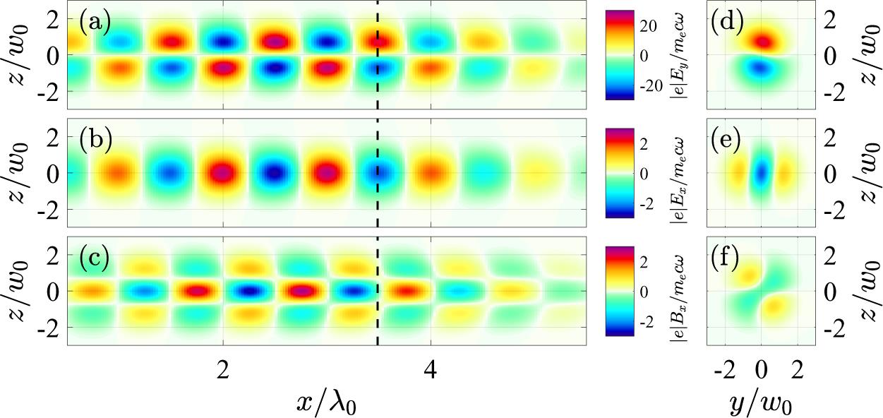
Fig. 1. Electric and magnetic field components of an LP-LG laser beam before it encounters the plasma. Panels (a) and (d) show ; panels (b) and (e) show ; panels (c) and (f) show . The left-hand column ((a)–(c)) shows the field structure in the -plane at . The right-hand column ((d)–(f)) shows the field structure in the -plane at the -position indicated with the dashed line in panels (a)–(c). All the snapshots are taken at fs from the simulation with parameters listed in Table 1.

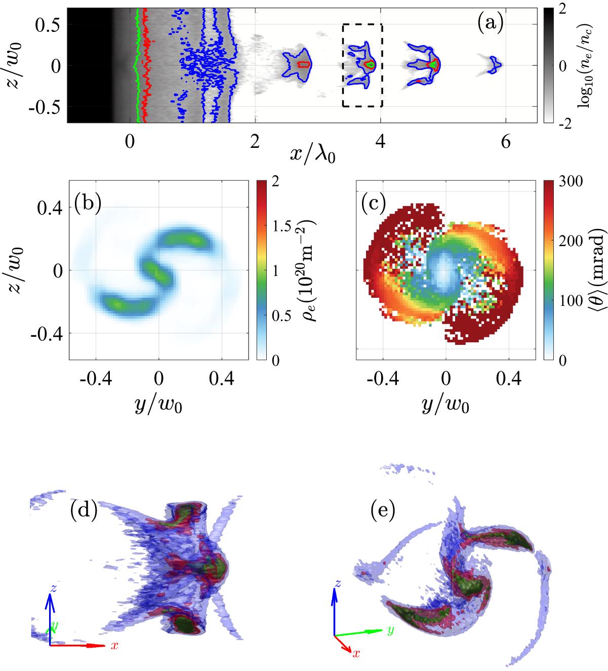
Fig. 2. Structure of electron bunches shortly after laser reflection off the plasma ( fs). (a) Electron density on a log-scale, with the color representing . The blue, red and green contours denote , and , respectively. The dashed rectangle marks the third bunch, whose additional details are provided in the remaining panels. (b) Electron areal density in the third bunch. (c) Cell-averaged electron divergence angle in the third bunch. (d), (e) 3D rendering of the electron density in the third bunch using different viewpoints.

Fig. 3. (a) Areal density of the electrons in the third bunch at time fs. (b) Three groups of electrons (blue, green and red markers) selected from the third bunch at fs for tracking. The electrons in each group are selected randomly. (c) Transverse positions of the three groups of electrons from (b) at fs. (d)–(f) Trajectories of the three groups of electrons in the transverse plane over the duration of the simulation. The line color shows electron energy. The markers show the electron locations at fs. (g)–(i) Time evolution of the longitudinal position for the same three groups of electrons, with (g) showing ‘blue’ electrons, (h) showing ‘green’ electrons and (i) showing ‘red’ electrons. The line color shows electron energy.

Fig. 4. Electric and magnetic fields after reflection of the LP-LG laser beam off the plasma. (a) Longitudinal profiles of the transverse electric field (red curve) and longitudinal magnetic field (blue line) at fs. Here, is plotted along the axis of the beam (, ), whereas is plotted at an off-axis location (, ) where its amplitude has the highest value. (b) Frequency spectra of (red line) and (blue line) from panel (a).

Fig. 5. Result of the long-term electron acceleration in the reflected LP-LG laser beam close to the beam axis. (a) Electron energy distribution as a function of at fs for electrons with . The inset shows the third bunch that is marked with the dashed rectangle in the main plot. (b) Time evolution of the electron distribution over the divergence angle in the third bunch (). (c) Time evolution of the electron energy spectrum in the third bunch. The black dashed curve is the prediction obtained from Equation (3) with . The start time of the acceleration is used as an adjustable parameter. (d) Electron energy versus the divergence angle in the third bunch shown in the inset of panel (a).

Fig. 6. (a) Areal density and (b) cell-averaged divergence angle in the cross-section of the third bunch at fs and . (c)–(e) Snapshots of the longitudinal electric field in the cross-section of the laser beam at , fs (c), , fs (d) and , fs (e). Here, is calculated using the analytical expression Equation (C28) given in Appendix C and is the amplitude of at , .

Table 1. 3D PIC simulation parameters. Here, m is the critical density corresponding to the laser wavelength . The initial temperatures for electrons and ions are set to zero.

Table 2. Parameters used for the four simulations depicted in Figure 7.

Table 3. Parameters of all five electron bunches at = 261 fs.