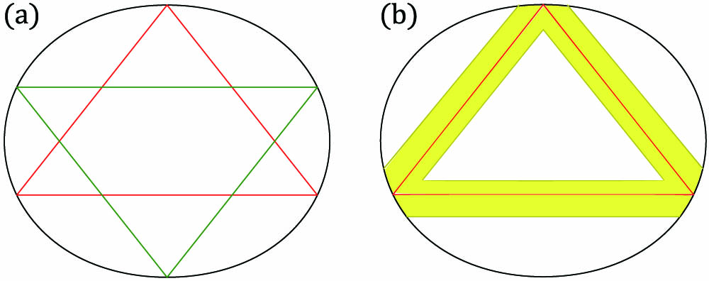
Fig. 1. (a) Double-triangle orbits in the quadrupole-deformed cavity. (b) Spatial selective pumping (yellow region) along the upward-pointing triangle orbit (red lines).

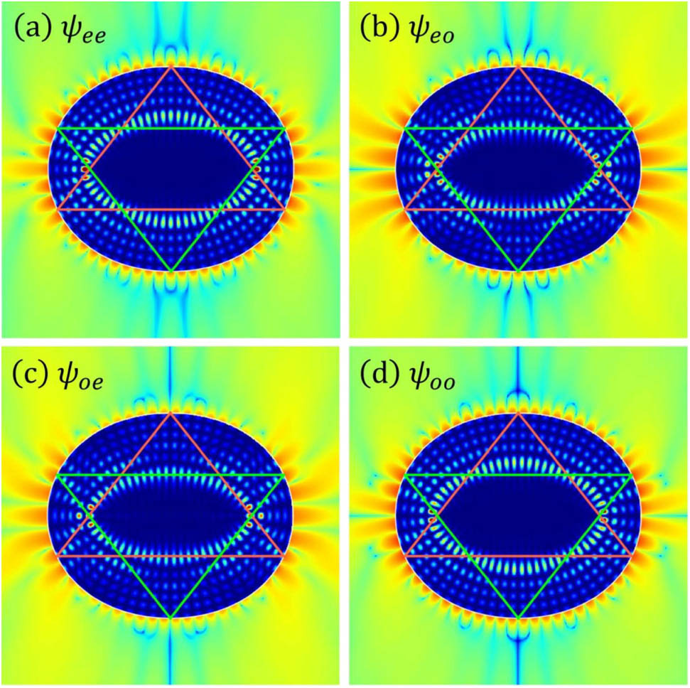
Fig. 2. Intensity distributions of the resonant modes for a passive quadrupole-deformed cavity with refractive index 3.3. The modes are four nearly degenerate modes associated with the double-triangle orbits. The double-triangle orbits (red and green lines) are superposed, and the intensities outside the cavity are plotted in log scale. (a) Even–even mode with scaled frequency Re ω/ω0=1.0008278. (b) Even–odd mode with Re ω/ω0=0.999085. (c) Odd–even mode with Re ω/ω0=0.999075. (d) Odd–odd mode with Re ω/ω0=1.0008277.

Fig. 3. Phase space of the ray dynamics for the quadrupole-deformed cavity. The islands of stability corresponding to the upward-pointing and downward-pointing triangle orbits are indicated by red and green points, respectively. The critical line for total internal reflection is indicated by a line at sin ϕ=1/3.3. Husimi distribution for the eo mode shown in Fig. 2(b) is superposed.

Fig. 4. Distribution of the complex eigenfrequencies ω scaled by ω0, where ω0 is the gain center parameter. The four nearly degenerate modes associated with the double-triangle orbits are encircled by a green circle (the ee and oo modes are almost on top of each other, and so are the eo and oe modes). The modes indicated by filled circles (•) have positive linear gain [i.e., satisfying Eq. (9)] for the selective pumping with W∞=1.0×10−3, whereas those indicated by crosses (×) do not satisfy Eq. (9).

Fig. 5. Electric field intensity distributions. (a) An initial condition for the MB model simulation. (b) Time-averaged pattern of the stationary lasing state of the MB model for the selective pumping case with W∞=1.0×10−3. The intensity outside the cavity is plotted in log scale. The boundary of the pumped area is indicated by yellow lines.

Fig. 6. Results of the MB model simulation for the selective pumping case with W∞=1.0×10−3. (a) Time evolution of the total light intensity inside the cavity. (b) Power spectrum of the electric field for the stationary lasing regime. The peak frequency is around ω/ω0=0.9988.

Fig. 7. Intensity distributions of the superpositions of the resonant-mode wave functions. The triangle orbit is indicated by red lines, and the intensities outside the cavities are plotted in log scale. (a) ξ=ψee+ψeo. (b) η=ψoe+ψoo. (c) ΨCW=ξ+iη=(ψee+ψeo)+i(ψoe+ψoo). (d) ΨCCW=ξ−iη=(ψee+ψeo)−i(ψoe+ψoo).

Fig. 8. Results of the MB model simulation for the uniform pumping case with W∞=3.0×10−4. (a) Time evolution of the total light intensity inside the cavity. (b) Power spectrum of the electric field for the stationary lasing regime. The frequencies of the primary and secondary peaks are ω/ω0≈0.9990 and ω/ω0≈1.0012, respectively.

Fig. 9. Time-averaged pattern of the stationary lasing state of the MB model for the uniform pumping case with W∞=3.0×10−4. The intensity outside the cavity is plotted in log scale.

Fig. 10. Intensity distribution of the superpositions of the resonant-mode wave functions. (a) ψeo+iψoe. (b) ψee+iψoo. The intensities outside the cavity are plotted in log scale.