
Zheng Sun, Minghui Duan, Yabing Zheng, Yi Jin, Xin Fan, Jinjin Zheng. Intensity diffusion: a concealed cause of fringe distortion in fringe projection profilometry[J]. Photonics Research, 2022, 10(5): 1210
- Photonics Research
- Vol. 10, Issue 5, 1210 (2022)
Abstract
1. INTRODUCTION
Due to their noncontact and high efficiency, optical three-dimensional (3D) measurement methods have high-impact applications in many fields [1], such as industrial product inspection [2–4], reverse engineering [5–7], and medical imaging [8,9]. Among these optical measurement methods, fringe projection profilometry (FPP) is one of the most promising techniques [10,11], in which the phase coding designed in fringe patterns plays an essential role in anti-interference [12]. For decoding the phase in fringe images, fringe analysis methods are subsequently developed and divided into spatial and temporal decoding methods. In spatial-decoding methods [13–19], the continuous phase map is computed from a single fringe pattern, which is applicable for measuring dynamic scenes [20,21]. The corresponding disadvantages are the loss of high-frequency 3D details and the failures in scenes consisting of isolated objects [22]. In temporal-decoding methods [23–31], the continuous phase map is obtained from the multiple fringe patterns, which can suppress the noise [32] and prevent the propagation of phase errors [30]. Therefore, temporal-decoding methods are more suitable for accurate 3D measurements.
In addition to fringe analysis methods, FPP’s performance is also dependent on the quality of fringe images. However, the nonlinear intensity response in the FPP system generally distorts the ideal fringes, thereby disrupting the phase distribution embedded in the fringe images. The known causes of fringe distortion include gamma distortion [33–38], residual high-order harmonics [39–42], and image saturation [43–48]. To cater to human visual perception, display devices introduce gamma distortion and generate a nonlinear response in the output intensity. However, this nonquantitative gamma transform causes unknown fringe distortion in the fringe images. Moreover, the high-order harmonic phenomenon is also a common source of fringe distortion. Especially in high-speed imaging techniques based on binary defocusing, the defocusing operation functions as a low-pass filter. When the degree of defocusing is insufficient, the high-order harmonics are not completely filtered out, and the residual harmonics distort the fringes. Image saturation means that the intensity of the image reaches the upper limit (255 in 8-bit gray level), which occurs because of the nonuniform scene reflectivity. The fringe information in the saturated regions is completely lost, thereby causing severe distortions in the fringe images.
To improve the quality of fringe images for 3D measurements, many researchers have proposed to correct the fringe distortion by considering the abovementioned causes. Replacing the digital projector with a liquid crystal projector [49,50], predistorting the designed fringes [36,51], and post-compensating for gamma-induced phase errors [34,52] are all valid measures for alleviating the impact of gamma distortion. For residual high-order harmonics, many studies [41,53] usually increase the frequency of harmonics to facilitate the effective operation of the low-pass filter. To avoid image saturation in multireflectivity scenes, researchers have tried to adjust the parameters of the FPP system, such as the exposure time and shoot number [43,46] or illumination intensity [48,54]. Researchers have made great efforts toward correcting the fringe distortion induced by these abovementioned causes, which makes it difficult to further improve the 3D measurement accuracy by optimizing the existing fringe distortion correction methods. Instead of continuing to optimize the existing fringe distortion correction methods, a concealed cause of fringe distortion, intensity diffusion, is revealed in this paper, which is generated because of the photocarrier diffusion between photodiodes (PDs) in the image sensors [55–62]. The photocarrier diffused from a pixel would be trapped by its neighboring pixels [57]. The trapped photocarrier is converted into the intensity, which represents the intensity diffused to the neighboring pixels. Moreover, the degree of diffusion depends on the pixel size [56,61], and the improvement in the resolution shrinks the pixel size, facilitating the diffusion. Facing the demand of high-resolution measurements, the intensity diffusion correction for FPP is significant.
Sign up for Photonics Research TOC. Get the latest issue of Photonics Research delivered right to you!Sign up now
The intensity diffused to the neighboring pixels is the nonlinear response to the illumination intensity output from the projector, thereby forming fringe distortion. The intensity diffused from one pixel to its neighbor is proportional to the pixel’s intensity and inversely proportional to the distance between the pixel and its neighbor [61]. Based on this analysis, the following characteristics of the fringe patterns would increase the impact of intensity diffusion. The first characteristic is the strong intensity contrast between the high-intensity area (HIA) and the low-intensity area (LIA) in one fringe pitch. The second characteristic is that an LIA is flanked by two HIAs. The former characteristic causes the intensity diffused from the HIA to have a great impact on the LIA. The latter indicates that the HIA is adjacent to the LIA, which further amplifies the impact of diffused intensity on the LIA. Moreover, the intensity contrast may be boosted with the increasing illumination intensity, and the distance between the HIA and LIA can be decreased with the increasing fringe frequency. In general, the intensity diffused from HIA to LIA results in a marked decline in the signal-to-noise ratio (SNR) of the fringe images. Therefore, removing the intensity diffusion distributed in the fringe images is a necessary but neglected task.
In this paper, we reveal that intensity diffusion induces a nonlinear response to the illumination intensity and mathematically explain how the diffused intensity distorts the fringe and reduces the SNR of the fringe image. Increasing the illumination intensity and fringe frequency is important for improving the 3D measurement accuracy. However, the intensity diffusion suppresses its improvement, and the effect of suppression is theoretically analyzed in this work. First, to implement accurate 3D profilometry, an intensity diffusion model (IDM) and an intensity diffusion correction algorithm (IDCA) are proposed to analyze and correct the fringe distortion, respectively. In the IDM, the effect of intensity diffusion is quantified based on the motion of photocarrier diffusion, and a diffusion coefficient is introduced to indicate the degree of intensity diffusion across adjacent pixels. Subsequently, a set of patterns with an array of bright spots is designed for projection. In the corresponding spot images, a phase-matching technique is applied to identify the pixels lighted by the illumination intensity and diffused intensity, and thereby the global diffusion coefficient distribution is determined based on the identified results. Finally, with the established IDM, the IDCA can remove the diffused intensity from the fringe images after calculating the specific value of the diffused intensity in each pixel. The fringe distortions and 3D measurement errors caused by intensity diffusion are experimentally shown to verify the necessity of removing the intensity diffusion. In addition, the experimental results show that the fringe images processed by IDCA can be used to retrieve more accurate 3D shapes.
2. PRINCIPLE
A. Illustration of the Intensity Diffusion
As displayed in Figs. 1(a) and 1(b), a couple of patterns are designed to illustrate the phenomenon of intensity diffusion, and the two designed patterns differ significantly in the central area. Subsequently, the patterns are projected onto the plane and captured as the corresponding images shown in Figs. 1(c) and 1(d). To further compare the two patterns and two images, the cross sections of Figs. 1(a)–1(d) are plotted in Figs. 1(e) and 1(f), respectively. It is worth noting that the intensity values of the regions surrounding the central areas in the two patterns are the same, whereas the intensity values of the corresponding regions of the two images are different. Considering that the plane is a standard matte ceramic plane with a uniform distribution of reflectivity, which successfully suppresses the disturbance of the interreflections, thus the primary factor causing this difference is intensity diffusion.
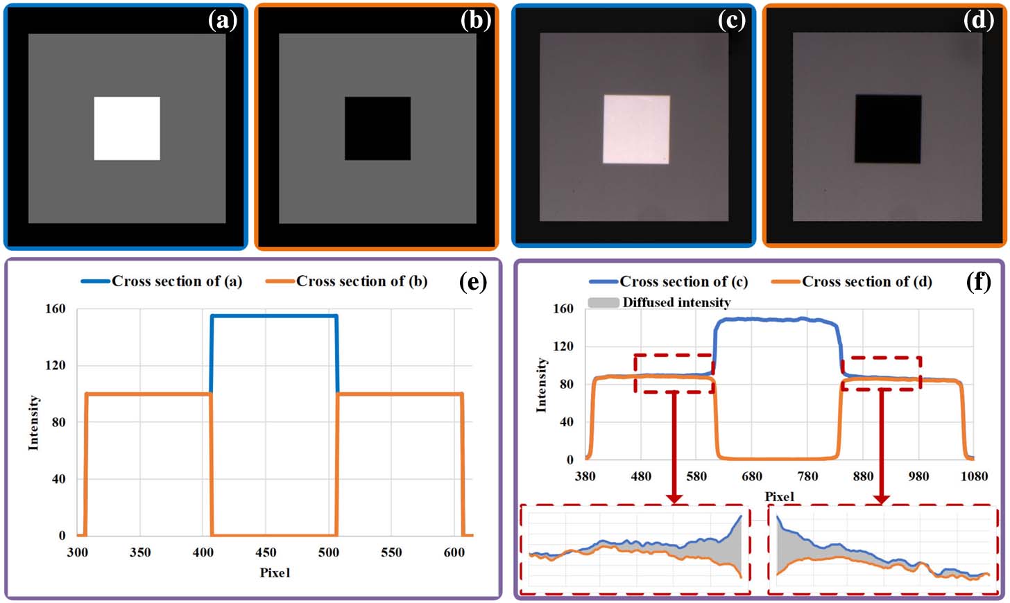
Figure 1.Illustration of the intensity diffusion. (a) Designed pattern. (b) Designed pattern without the central area. (c) The image of (a). (d) The image of (b). (e) Cross sections of the patterns in (a) and (b). (f) Cross sections of the images in (c) and (d).
According to existing studies [57,60,61], the value of the intensity diffused from a pixel to its neighboring pixels is determined by the intensity of the pixel and the distance between the pixel and its neighbor. To simplify the subsequent analysis, the pixel and its neighbor are named the diffused source (DS) and diffused target (DT), respectively. Figure 1(f) indicates that the diffused intensity attenuates with the increasing distance between the DS and the DT. To quantify the attenuation trend, the diffusion coefficient is adopted. The diffused intensity in the DT (i.e., ) can be expressed as
B. Influence of the Diffused Intensity on the Fringe Pattern
The influence of intensity diffusion on the fringe pattern includes a reduction in the SNR of fringe images and a suppression of the accuracy improvement achieved by increasing the illumination intensity and fringe frequency.
The visual impact of the intensity diffusion is fringe distortion as shown in Fig. 2. Compared to gamma distortion, high-order harmonics, and image saturation, the waveform of the fringe distorted by intensity diffusion is still close to a sinusoidal distribution. However, the variation of intensity diffusion is nonuniform, introducing a nonlinear response in the intensity of fringes, and thus the effect of intensity diffusion cannot be ignored, particularly for LIAs in a fringe pitch.
![]()
Figure 2.Fringe distortions induced by intensity diffusion, gamma distortion, high-order harmonics, and image saturation.
In the projection space, the fringe pattern can be expressed as
As shown in Fig. 2, the LIA can be regarded as the diffused target of the HIA, and in LIA (i.e., ) can be described as
To simplify Eq. (5), we propose two assumptions as follows. 1) Assuming , ensuring that the modulation (i.e., ) is maximized, the illumination intensity can be adjusted by changing . 2) Assuming , the illumination intensity is equivalently transformed into the reflected intensity. In addition to the diffused intensity, the random noise is also a part of the intensity of the fringe image (i.e., the captured intensity ), which can be expressed as
According to Eq. (7), the reflection of the illuminated light is taken as the signal part of the image, whereas the other terms are regarded as noise. Considering that is much lower than , the diffused intensity determined by heavily reduces , further decreasing the 3D measurement accuracy. To improve the 3D measurement, it is common to increase the illumination intensity (i.e., increasing ). Equation (7) indicates that is a monotone increasing function, and the second derivative of is expressed as
Equation (8) shows that , and thus is a decreasing function, which means that the growth rate of decreases with increasing . Similarly, without the diffused intensity is expressed as
According to Eq. (9), is equal to 0, and thus the growth rate of is constant with increasing . Equations (8) and (9) demonstrate that the diffused intensity suppresses the growth rate of when increasing the illumination intensity. To further analyze the suppression, the relationship between and the proportion of the diffused intensity in the captured intensity is expressed as
Moreover, the derivative of is expressed as
Equations (10) and (11) show that is an increasing function, and the proportion of diffused intensity in the captured intensity rises with increasing , thereby limiting the improvement in the SNR.
Apart from increasing the illumination intensity, increasing the fringe frequency is another necessary procedure for improving the 3D measurement accuracy. However, the increase in the fringe frequency also shortens the distance between the HIAs and LIAs. The analysis developed in Section 2.A demonstrates that the DT’s diffusion coefficient increases with decreasing distance between the DS and DT. The relationship between and is expressed as , and the derivative of is expressed as
In conclusion, intensity diffusion induces fringe distortion in the images and reduces their SNRs, particularly in LIAs. Apart from that, the two important procedures for improving the 3D measurement accuracy are both limited by intensity diffusion. The SNR indeed improves with increasing illumination intensity, but the improvement is hampered because the proportion of the diffused intensity in the captured intensity also increases as demonstrated in Eqs. (10) and (11). Increasing the fringe frequency improves the 3D measurement accuracy [30] by expanding the phase range, but it shortens the distance between the HIAs and LIAs, enlarging the LIA’s diffusion coefficient. According to Eq. (12), the enlarged diffusion coefficient reduces the SNR. Meanwhile, the reduction in the SNR also decreases with the increasing fringe frequency, which is demonstrated in Eq. (13), indicating that the influence of the intensity diffusion attenuates with the increasing fringe frequency.
C. Phase Errors Induced by the Intensity Diffusion
Fourier transform profilometry (FTP) [63] and the phase-shifting algorithm (PSA) [24] are two typical methods for retrieving the wrapped phase distribution from fringe images. In FTP, the single fringe pattern can be described as
D. Unwrapping Errors Induced by the Intensity Diffusion
After retrieving the wrapped phase, all the phase values are within in the phase domain, and thus eliminating discontinuity is an essential process. Compared with spatial phase unwrapping methods, temporal phase unwrapping (TPU) methods can handle discontinuous surfaces [26] and suppress the propagation of noise-induced errors [25]. In TPU, the discontinuity is eliminated by the fringe order, which is often encoded in the additional information, such as the gray code [27] and additional fringe patterns [29,31]. Compared with the gray code, the additional fringe patterns have advantages of pattern efficiency, unambiguous range, and unwrapping accuracy [30]. Figure 3 shows the flow chart of the phase coding unwrapping (PCU) method and multifrequency unwrapping (MFU) method, which calculate the fringe order accurately by projecting additional fringe patterns. The discontinuity is removed by adding multiple in each pixel, and the relationship between the wrapped phase and the unwrapped phase can be expressed as
![]()
Figure 3.Illustration of the TPU methods based on additional fringe patterns.
In the PCU, the ancillary phase map extracted from the additional fringe images is a stair phase distribution, and the fringe order is calculated by
In MFU, the ancillary phase map is a low-frequency phase distribution, and the fringe order in MFU is expressed as
To explore whether the PCU or MFU is more sensitive to phase errors, the difference between and is described as
The relationship between the fringe frequencies in the PCU and MFU is known (i.e., ). Based on this relationship and Eq. (12), the SNR of the fringe images in the PCU is lower than that in the MFU. Following that, according to Eq. (19), is larger than . Substituting the above conditions into Eq. (24), it can be deduced that . Therefore, PCU is more sensitive to phase errors, indicating that the intensity diffusion has a greater impact on PCU.
3. PROPOSED METHOD
The proposed method includes establishing a mathematical model (i.e., IDM) for quantifying the intensity diffusion in the fringe images and developing an iteration algorithm (i.e., IDCA) to calculate the diffused intensity in each pixel and remove it from the fringe images.
A. Intensity Diffusion Model
As indicated in Fig. 4, the intensity diffusion in the pixel area is caused by photocarrier diffusion between PDs, and the key procedure for establishing IDM is determining the diffusion coefficient for each pixel, which can be calculated by
![]()
Figure 4.Illustration of the parameters in IDM.
To obtain and for a given fringe projection system (FPS), a set of patterns with an array of spots is designed. These patterns consist of 256 bright spots, which correspond to 8-bit gray level. As shown in Fig. 5, the patterns with spots are projected onto a standard matte ceramic plane with a flatness of 4.4 μm and measurement uncertainty of 0.8 μm. In the images with spots, the pixels are lighted not only by the illumination intensity but also by the diffused intensity. Therefore, to distinguish whether the pixels are lighted by the illumination intensity or the diffused intensity, it is necessary to build the correspondence between the projection space and the imaging space. As a result, the coordinate mapping technique is performed by a phase-matching algorithm [48], which can simply be denoted as
![]()
Figure 5.Flow chart of the proposed method. (a) Procedures of establishing IDM. (b) Process of IDCA.
B. Intensity Diffusion Correction Algorithm
The global diffusion coefficient distribution is determined after obtaining and , and then the diffused intensity in each pixel can be calculated by
However, in the fringe image, the reflected intensity in each pixel is unknown. Therefore, the captured intensity is taken as the initial reflected intensity to calculate the initial diffused intensity (i.e., ). Then an iteration operation is adopted to accurately calculate as shown in Fig. 5(b). The captured intensity is larger than the reflected intensity, and thus the transmission from to is a decreasing process. To meet this condition, the iteration operation should stop when , and the iteration-stopping criterion [i.e., in Fig. 5(b)] is set as zero. After iteration, is taken as the value of final diffused intensity, which is subtracted from the value of captured intensity.
4. EXPERIMENT AND ANALYSIS
To present the influence of intensity diffusion and validate the proposed method, we built an FPS consisting of a projector with a resolution (Texas Instruments, DLP 4500) and an industrial camera with a resolution (PointGrey, Grasshopper3). The experiment includes four parts. The first part is conducted to show the fringe distortion induced by the intensity diffusion and verify the effectiveness of the IDCA on removing the diffused intensity. The second part presents the improvement in 3D measurement accuracy by the IDCA. The third part further shows the IDCA’s enhancement of the accuracy improvement approaches. The fourth part shows the ability of the IDCA to reduce the errors in the measurement tasks of the high-contrast and high-reflectivity scenes.
A. Fringe Distortion by the Intensity Diffusion
Two groups of fringe patterns are designed to show the fringe distortion caused by the intensity diffusion. The first group includes three sinusoidal fringe patterns () with different illumination intensities, which are used to show the variation in the intensity diffusion with the increasing illumination intensity. The illumination intensities of the three fringe patterns are set as 24%, 36%, and 54% of the maximum illuminance of the projector light source. The cross sections of the corresponding fringe images are shown in Figs. 6(a)–6(c). The second group includes three sinusoidal fringe patterns with different fringe frequencies, which are used to show the variation in the intensity diffusion with the increasing fringe frequency. The fringe frequencies of the three fringe patterns are set as 32, 64, and 128. The cross sections of the corresponding fringe images are shown in Figs. 6(d)–6(f).
![]()
Figure 6.Cross sections of the fringes distorted by the intensity diffusion and the corresponding results corrected by IDCA. (a) Fringe with 40% of maximum illumination intensity. (b) Fringe with 50% of maximum illumination intensity. (c) Fringe with 60% of maximum illumination intensity. (d) Fringe with a fringe frequency of 32. (e) Fringe with a fringe frequency of 64. (f) Fringe with a fringe frequency of 128.
To avoid the coupling of the fringe distortions induced by multiple causes, first, the fringe patterns are predistorted by a reciprocal of the gamma value (i.e., ) to compensate for the gamma distortion. Second, the fringe patterns are designed as 8-bit sinusoidal fringe patterns for preventing high-order harmonics. Finally, to avoid image saturation, fringe patterns are projected onto a plane with uniform reflectivity.
To underline the fringe distortion induced by intensity diffusion, the referenced fringes are designed, which are least-squares fitting results of the cross sections of fringe images. In addition, two key measures are required to reduce the difference between the referenced fringes and the ground truths as follows. (1) The projection object should be a standard plane with sufficiently high flatness, which can reduce the disturbance of fringe deformation. (2) A two-dimensional (2D) image of the plane is recorded before projection. In the 2D image, the area with the smallest intensity gradient is marked, and only the fringes in the marked area are selected to be fitted for minimizing the disturbance of reflectivity.
Figures 6(a)–6(c) show the cross sections of the fringes with different illumination intensities. Compared with the referenced fringes, there are bulges on the crests and troughs that are not supposed to appear. Since the other three causes of fringe distortion have been avoided, these bulges are primarily induced by intensity diffusion. Equation (5) indicates that increasing the illumination intensity increases the diffused intensity; however, the captured intensity also increases, which alleviates the aggravation of the fringe distortion. Therefore, increasing the illumination intensity is still a suitable approach for suppressing the fringe distortion. Figures 6(d)–6(f) show the cross sections of the fringes with different fringe densities, and the bulges on crests and troughs are more distinct when compared with those in Figs. 6(a)–6(c). As discussed in Section 2, the increase in fringe frequency shortens the distance between the HIAs and LIAs, and it decreases the modulation in the illumination intensity, thereby aggravating the fringe distortion. As the fringe frequency reaches 128, the bulges on the crests and troughs become prominent, and the waveforms of the cross sections are uneven. Therefore, increasing the fringe frequency should not be the primary approach for improving the 3D measurement accuracy when the given FPS has a large initial diffusion coefficient (i.e., ). After removing the diffused intensity by IDCA, the bulges are removed, and the uneven waveforms are corrected.
B. Improvement in the 3D Measurement Accuracy by IDCA
To demonstrate the IDCA’s improvement in the 3D measurement accuracy, two standard objects are taken as the experimental objects. In the 3D reconstruction of the standard objects, the phase is retrieved by the three-step PSA, and the retrieved phase is unwrapped by the multi-frequency unwrapping method [28]. The phase retrieval method uses three fringe patterns with a phase shift of , and the corresponding fringe frequency is 56. The process of phase unwrapping uses two sets of fringe patterns. The first set includes three fringe patterns with a phase shift of , and the corresponding fringe frequency is 1. The second set includes three fringe patterns with a phase shift of , and the corresponding fringe frequency is 16.
To further verify the improved 3D measurement accuracy of the IDCA, four cases are designed. denotes that the IDCA is not applied to any fringe images, denotes that the IDCA is only applied to the six fringe images for phase unwrapping, denotes that the IDCA is only applied to the three fringe images for phase retrieval, and denotes that the IDCA is applied to all fringe images. The 3D reconstruction results in Figs. 7(b)–7(e) correspond to the four cases, respectively. To visually show the quality of the 3D reconstruction results, the deviations between the reconstructed planes and the least-squares fitting planes are calculated, and the degree of deviation is displayed by the colormap. The flatness of the standard plane is only 4.4 μm (), which is close to a perfect plane. Therefore, the least-squares fitting plane can be regarded as the ground truth of the reconstructed result, and the 3D measurement accuracy is inversely proportional to the deviations. The decrease in the deviation from Fig. 7(b) to Fig. 7(e) demonstrates that the application of IDCA improves the 3D measurement accuracy. To further show the reduction of the deviation by IDCA, the cross sections of the reconstructed planes are displayed in Fig. 7(f), and the corresponding local enlargement is also shown in Fig. 7(g). Compared with the cross sections of other cases, the fluctuation of is smaller, which proves the effectiveness of IDCA in improving the 3D measurement accuracy.
![]()
Figure 7.3D reconstruction results of the standard plane in the four cases. (a) Normal image of the standard plane. (b) 3D reconstruction result in the case of
Figure 8 shows the 3D reconstruction results of the standard sphere. The 3D reconstruction results in Figs. 8(b)–8(e) also correspond to the four cases. Similar to the reconstructed planes, the colormap displays the degree of deviation between the reconstructed spheres and the least-squares fitting spheres. The roundness of the standard sphere is only 2.6 μm (), which is beyond the range of measurement accuracy of FPS. Therefore, the least-squares fitting sphere can be regarded as the ground truth of the reconstructed result. The decrease in the deviation from Fig. 8(b) to Fig. 8(e) also demonstrates that the application of IDCA improves the 3D measurement accuracy. In Figs. 8(f) and 8(g), the cross sections of the reconstructed spheres and the corresponding local enlargement also show that the fluctuation of the reconstructed surface significantly decreases after the application of IDCA. Moreover, by comparing the cross sections of with the cross sections of in Figs. 7(g) and 8(g), the fluctuation of the cross sections of is larger than the fluctuation of the cross sections of . The results indicate that the phase retrieval method with IDCA is significantly improved compared with the phase unwrapping method.
![]()
Figure 8.3D reconstruction results of the standard sphere in the four cases. (a) Normal image of the standard sphere. (b) 3D reconstruction result in the case of
To further show the accuracy improvement by IDCA, four different combinations between the phase retrieval methods and phase unwrapping methods are developed. The first combination includes FTP and PCU, the second includes FTP and MFU, the third includes PSA and PCU, and the fourth includes PSA and MFU. In these combinations, FTP uses a single sinusoidal fringe pattern with a fringe frequency of 56, and the PSA uses three sinusoidal fringe patterns with a fringe frequency of 56 and a phase shift of . PCU [29] uses two sets of stair phase-encoded fringe patterns to generate two additional stair phase maps for calculating the fringe order. The first set includes three fringe patterns with a fringe frequency of 1 and a phase shift of , and the second set includes three fringe patterns with a fringe frequency of 16 and a phase shift of . MFU [28] uses two sets of sinusoidal fringe patterns to generate two additional periodic phase maps for calculating the fringe order. The first set includes three fringe patterns with a fringe frequency of 1 and a phase shift of , and the second set includes three fringe patterns with a fringe frequency of 16 and a phase shift of .
To quantitatively present the IDCA’s improvement in the 3D measurement accuracy, the root-mean-square errors (RMSEs) of the reconstructed plane and sphere are calculated. RMSEs are the root-mean-square values of the deviations between the reconstructed 3D profiles and the corresponding least-squares fitting 3D profiles, and the deviation of each point on the reconstructed 3D profiles is the distance between the point and the corresponding point on the least-squares fitting 3D profiles. The flatness of the standard plane is 4.4 μm (), and the roundness of the reconstructed sphere is 2.6 μm (), which are given by the calibration report from the National Hi-tech Metrology Station in Shenzhen, China. The flatness and the roundness are both beyond the range of the measurement accuracy of the fringe projection system; thus, the ground truths of the reconstructed 3D profiles can be regarded as the perfect plane and sphere. The least-squares fitting results of the reconstructed 3D profiles are also the perfect plane and sphere. Therefore, the least-squares fitting 3D profiles are regarded as the ground truths for evaluating the accuracy of 3D reconstruction.
Table 1 lists the RMSEs in the four cases of each combination, as well as the reduction rate of RMSE corresponding to the case of . Among the four cases, the RMSE reduction rate in the case of is the highest, indicating that the accuracy improvement is the largest when IDCA is applied to both the phase retrieving and phase unwrapping methods. The case of has a lower reduction rate of RMSE than that in the case of , which indicates that the phase unwrapping method achieves a minor accuracy improvement compared with the phase retrieval method. Therefore, the phase unwrapping method is less sensitive to the phase errors induced by the intensity diffusion. Equation (24) indicates that MFU has a better tolerance for phase errors compared with PCU; therefore, MFU also achieves a minor accuracy improvement. Accuracies of the 3D Measurement Results in Four CombinationsRMSE (μm) and the Corresponding Reduction Rate Object IDCA [−,−] IDCA [−,+] IDCA [+,−] IDCA [+,+] IDCA [−,−] IDCA [−,+] IDCA [+,−] IDCA [+,+] Plane 138.43 127.95 123.86 117.45 128.70 121.78 116.01 111.53 0.00% 7.57% 10.52% 15.16% 0.00% 5.38% 9.86% 13.33% Sphere 218.94 201.31 187.74 179.16 201.33 189.59 174.96 168.01 0.00% 8.05% 14.25% 18.17% 0.00% 5.83% 13.09% 16.55% Plane 40.21 37.55 36.37 34.93 38.18 36.01 35.03 33.48 0.00% 6.64% 9.55% 13.14% 0.00% 5.67% 8.25% 12.32% Sphere 60.15 56.22 53.97 51.38 56.12 53.38 50.79 48.46 0.00% 6.52% 10.26% 14.57% 0.00% 4.88% 9.49% 13.66%
To analyze the accuracy improvement of the IDCA with the increase in fringe frequencies, the combination of PSA and MFU [28] is selected to calculate the RMSEs when the fringe frequency increases from 32 to 80, and the corresponding RMSEs are listed in Table 2. As discussed in Section 2, the increase in the fringe frequency reduces the SNR of the fringe images, and thus the reduction rate of the RMSE should rise with the increase in the fringe frequency. However, in the part of the plane, the reduction rate of the RMSE decreases as the fringe frequency increases from 32 to 56, indicating that the impact of the intensity diffusion on the accuracy attenuates with the increasing fringe frequency. Consequently, the experimental results are consistent with the conclusion of Eq. (13), i.e., the reduction in the SNR induced by intensity diffusion attenuates with the increase in the fringe frequency. Meanwhile, the reduction rate of RMSEs starts to rise once the fringe frequency reaches 64. Considering that the modulation attenuation with the increase in the fringe frequency is nonlinear, the rapidly decreasing modulation amplifies the impact of intensity diffusion when the fringe frequency reaches 64, and then the reduction rate of RMSEs rises as the fringe frequency increases from 64 to 80. As a result, with the assistance of the IDCA, increasing the fringe frequency is still an effective approach for improving the 3D measurement accuracy. Accuracy Improvement with Different Fringe FrequenciesFringe Frequency Plane Sphere RMSE (μm) Reduction Rate RMSE (μm) Reduction Rate IDCA[−,−] IDCA[+,+] IDCA[−,−] IDCA[+,+] 42.00 36.59 12.87% 63.46 54.78 13.68% 40.71 36.77 12.63% 60.44 52.38 13.34% 39.46 34.55 12.45% 58.12 50.49 13.12% 38.18 33.48 12.32% 56.12 48.46 13.66% 36.94 32.24 12.72% 53.64 46.07 14.11% 34.62 30.03 13.27% 49.11 41.85 14.79% 31.60 27.34 13.49% 47.44 40.16 15.35%
C. IDCA’s Performance on the Accuracy Improvement
Increasing the illumination intensity and increasing the fringe frequency are two necessary procedures for improving the 3D measurement accuracy [30,32]. However, Eqs. (8) and (11) demonstrate that the increase in illumination intensity increases the proportion of the diffused intensity in the fringe images, suppressing the improvement in the 3D measurement accuracy. Equation (12) indicates that the increase in the fringe frequency directly reduces the SNR of the fringe images, which also suppresses the accuracy improvement. To verify the feasibility of the IDCA from the two perspectives, the variations in RMSEs with the increase of the illumination intensity and fringe frequency are shown in Fig. 9.
![]()
Figure 9.3D measurement accuracy for the plane and sphere with different illumination intensities and fringe frequencies. (a) Reciprocals of RMSE with the increasing illumination intensity. (b) Gradient of 1/RMSE with the increasing illumination intensity. (c) Reciprocal of RMSE with the increasing fringe frequency. (d) Gradient of 1/RMSE with the increasing fringe frequency.
Figure 9(a) plots the reciprocal of the RMSE (i.e., 1/RMSE) obtained when the illumination intensity increases from (24% of the maximum illumination intensity). In the reconstruction in Fig. 9(a), the phase retrieval method uses three sinusoidal fringe patterns () with a phase shift of . The phase unwrapping method uses two sets of sinusoidal fringe patterns; the first set includes three fringe patterns () with a phase shift of , and the second set includes three fringe patterns () with a phase shift of . The RMSEs in Fig. 9(a) decrease with the increasing illumination intensity, which indicates that increasing the illumination intensity can continuously improve the 3D measurement accuracy before image saturation occurs. The gradient of 1/RMSE in Fig. 9(b) continuously decreases, which means that the accuracy improvement decreases. As analyzed by Eq. (9), the diffused intensity increases with increasing illumination intensity, thereby hampering the accuracy improvement. After removing the diffused intensity by the IDCA, the gradient of 1/RMSE increases, indicating that the accuracy improvement is enhanced.
Figure 9(c) plots 1/RMSE obtained when the fringe frequency increases. As mentioned in Section 1 the accuracy improves because the increase in the fringe frequency expands the phase coding range. However, Eq. (12) indicates that the increase in the fringe frequency also reduces the SNR of the fringe images. Moreover, the projector defocusing causes a significant attenuation of the modulation. As shown in Fig. 9(c), when the fringe frequency reaches a certain value, the RMSE starts to increase. Therefore, improving the SNR of the fringe images is essential for high-frequency fringe images. After removing the diffused intensity by IDCA, the critical point between the decrease and increase in RMSE is delayed, increasing the upper limit of fringe frequency by 18.2% and 20% for measuring the plane and sphere, respectively.
D. Measuring the Scenes with High Contrast and High Reflectivity
The high contrast in the scene can enlarge the impact of intensity diffusion on reducing the SNR of the fringe image. The waveforms plotted in Fig. 10 show the fringes in the boundary areas between the black and white regions. The intensity values of the white regions are much higher than those of the black regions, enlarging the proportion of diffused intensity in the intensity of the black region. Therefore, the SNR of the black region is heavily reduced, thereby resulting in serious phase errors. To depict the errors induced by the high contrast, the zebra and panda models are taken as the experimental objects.
![]()
Figure 10.Fringe images in the scenes with high contrast.
Figure 11 displays the unwrapped phase maps of the two models obtained by the combination of PSA and MFU [28], which uses three sets of sinusoidal fringe patterns with a phase shift of . The first set includes three fringe patterns with a fringe frequency of 56, the second set includes three fringe patterns with a fringe frequency of 1, and the third set includes three fringe patterns with a fringe frequency of 16. In the case of , as shown in Figs. 11(a) and 11(e), there are serious phase errors in the areas with the high contrast and the background surrounding models. As shown in Figs. 11(b) and 11(f), the phase errors in the areas with the high contrast are significantly reduced after the IDCA is applied to the phase retrieval procedure. Figures 11(c) and 11(g) show the results when IDCA is merely applied to the phase unwrapping method, and the phase errors are still apparent. Therefore, the phase errors induced by the intensity diffusion mainly occur in the phase retrieval procedure. The phase errors in the case of are significantly reduced as illustrated in Figs. 11(d) and 11(h). In addition, the remaining phase errors in the background can be removed by a threshold segmentation operation [64]. However, as shown in Fig. 10, the segmentation operation indiscriminately removes both the black regions on the model and the background in the actual scene. Therefore, improving the SNR of the background is the primary goal for measuring the scenes with high contrast.
![]()
Figure 11.Unwrapped phase maps of the panda and zebra models. (a)–(d) Unwrapped phase maps of the panda model in the four cases. (e)–(h) Unwrapped phase maps of the zebra model in the four cases.
The high reflectivity in the scene can also enlarge the impact of intensity diffusion. The waveforms plotted in Fig. 12(b) show the cross sections of the fringes in the high-reflectivity regions. The intensity values of high-reflectivity regions are close to the upper limit of intensity, which could result in errors in the 3D reconstruction results. Moreover, the intensity diffused from the crest of fringes greatly impacts the trough of fringes, which heavily reduces the SNRs of the trough of fringes. To show the improvement in 3D reconstruction accuracy by IDCA in the high-reflectivity scene, the steel plate is taken as the experimental object.
![]()
Figure 12.3D reconstruction results of the steel plate. (a) Normal image of the steel plate. (b) Cross sections of the fringes in the high-reflectivity areas. (c) Image of the steel plate with fringes. (d) 3D reconstruction result in the case of
Figure 12 displays the 3D reconstruction results of the steel plate, which are also obtained by the combination of three-step PSA and MFU [28]. The fringe frequencies of the three sets of sinusoidal fringe patterns used are 1, 16, and 56. The degree of deviation between the reconstructed plate and the least-squares fitting plate is also expressed by the colormap. As shown in Figs. 12(d)–12(g), the deviation decreases with the application of IDCA, which indicates that the 3D measurement accuracy is improved. As discussed above, the intensity diffused from the crest of fringes greatly reduces the SNRs of the trough of fringes, which cause a ripple on the high-reflectivity region on the reconstructed surface as shown in Fig. 12(d). Similar to the decrease in deviation, the ripple is also removed with the application of IDCA.
E. Limitation of the Proposed Method
The main limitations of the proposed method are discussed as follows. Number of Iterations in the IDCA and the Corresponding RMSEsNumber of Iterations RMSE (μm) 0 35.87 34.14 1 35.39 33.82 2 35.10 33.67 3 34.93 33.48 4 34.83 33.55 5 34.84 33.52
5. CONCLUSION
In this paper, we reveal a factor that causes fringe distortions in FPP: intensity diffusion. The factor has been neglected in the existing research on fringe distortion correction. The analysis of intensity diffusion indicates that the diffused intensity nonuniformly increases the intensity of the fringe images and reduces the SNRs of the fringe images. Moreover, the intensity diffusion suppresses the effectiveness of increasing illumination intensity and fringe frequency, which hampers the accuracy improvement. To improve the quality of the fringe images, the IDM is established to quantify the intensity diffusion in the fringe images. Then, the IDCA is presented to eliminate the diffused intensity. By utilizing the proposed method, the fringe distortion caused by intensity diffusion is effectively corrected. Theoretically and experimentally, the intensity diffusion is a significant cause of fringe distortions, which should not be neglected in the research about FPP. With the proposed methods, the quality of the fringe images can be improved, and the advantage of FPP in reconstructing high-precision 3D shape profilometry is consolidated.
References
[1] F. Chen, G. M. Brown, M. Song. Overview of 3-D shape measurement using optical methods. Opt. Eng., 39, 10-22(2000).
[2] R. Usamentiaga, J. Molleda, D. F. García. Fast and robust laser stripe extraction for 3D reconstruction in industrial environments. Mach. Vis. Appl., 23, 179-196(2012).
[3] T. Zhang, J. Liu, S. Liu, C. Tang, P. Jin. A 3D reconstruction method for pipeline inspection based on multi-vision. Measurement, 98, 35-48(2017).
[4] P. Rodríguez-Gonzálvez, M. Rodríguez-Martín, L. F. Ramos, D. González-Aguilera. 3D reconstruction methods and quality assessment for visual inspection of welds. Autom. Constr., 79, 49-58(2017).
[5] J. Burke, T. Bothe, W. Osten, C. F. Hess. Reverse engineering by fringe projection. Proc. SPIE, 4778, 312-324(2002).
[6] G. Sansoni, F. Docchio. Three-dimensional optical measurements and reverse engineering for automotive applications. Robot. Comput.-Integr. Manuf., 20, 359-367(2004).
[7] J. Hecht, K. Lamprecht, M. Merklein, K. Galanulis, J. Steinbeck. Triangulation based digitizing of tooling and sheet metal part surfaces-measuring technique, analysis of deviation to CAD and remarks on use of 3D-coordinate fields for the finite element analysis. Key Engineering Materials, 344, 847-853(2007).
[8] K. R. Ford, G. D. Myer, T. E. Hewett. Reliability of landing 3D motion analysis: implications for longitudinal analyses. Med. Sci. Sports Exercise, 39, 2021-2028(2007).
[9] U. Khan, A. Yasin, M. Abid, I. Shafi, S. A. Khan. A methodological review of 3D reconstruction techniques in tomographic imaging. J. Med. Syst., 42, 192(2018).
[10] S. S. Gorthi, P. Rastogi. Fringe projection techniques: whither we are?. Opt. Laser Eng., 48, 133-140(2010).
[11] Z. Wu, W. Guo, Y. Li, Y. Liu, Q. Zhang. High-speed and high-efficiency three-dimensional shape measurement based on gray-coded light. Photon. Res., 8, 819-829(2020).
[12] S. Feng, C. Zuo, L. Zhang, W. Yin, Q. Chen. Generalized framework for non-sinusoidal fringe analysis using deep learning. Photon. Res., 9, 1084-1098(2021).
[13] M. Takeda, K. Mutoh. Fourier transform profilometry for the automatic measurement of 3-D object shapes. Appl. Opt., 22, 3977-3982(1983).
[14] J. Zhong, J. Weng. Spatial carrier-fringe pattern analysis by means of wavelet transform: wavelet transform profilometry. Appl. Opt., 43, 4993-4998(2004).
[15] L. Huang, Q. Kemao, B. Pan, A. K. Asundi. Comparison of Fourier transform, windowed Fourier transform, and wavelet transform methods for phase extraction from a single fringe pattern in fringe projection profilometry. Opt. Laser Eng., 48, 141-148(2010).
[16] R. Goldstein, H. Zebker, C. Werner. Satellite radar interferometry: two-dimensional phase unwrapping. Radio Sci., 23, 713-720(1988).
[17] D. C. Ghiglia, L. A. Romero. Minimum LP-norm two-dimensional phase unwrapping. J. Opt. Soc. Am. A, 13, 1999-2013(1996).
[18] T. J. Flynn. Two-dimensional phase unwrapping with minimum weighted discontinuity. J. Opt. Soc. Am. A, 14, 2692-2701(1997).
[19] R. Bamler, P. Hartl. Synthetic aperture radar interferometry. Inverse Prob., 14, R1(1998).
[20] X. Su, W. Chen, Q. Zhang, Y. Chao. Dynamic 3-D shape measurement method based on FTP. Opt. Laser Eng., 36, 49-64(2001).
[21] X. Su, Q. Zhang. Dynamic 3-D shape measurement method: a review. Opt. Laser Eng., 48, 191-204(2010).
[22] Y. Hu, Q. Chen, S. Feng, C. Zuo. Microscopic fringe projection profilometry: a review. Opt. Laser Eng., 135, 106192(2020).
[23] V. Srinivasan, H.-C. Liu, M. Halioua. Automated phase-measuring profilometry of 3-D diffuse objects. Appl. Opt., 23, 3105-3108(1984).
[24] C. Zuo, S. Feng, L. Huang, T. Tao, W. Yin, Q. Chen. Phase shifting algorithms for fringe projection profilometry: a review. Opt. Laser Eng., 109, 23-59(2018).
[25] J. M. Huntley, H. Saldner. Temporal phase-unwrapping algorithm for automated interferogram analysis. Appl. Opt., 32, 3047-3052(1993).
[26] H. O. Saldner, J. M. Huntley. Temporal phase unwrapping: application to surface profiling of discontinuous objects. Appl. Opt., 36, 2770-2775(1997).
[27] G. Sansoni, M. Carocci, R. Rodella. Three-dimensional vision based on a combination of gray-code and phase-shift light projection: analysis and compensation of the systematic errors. Appl. Opt., 38, 6565-6573(1999).
[28] J. Tian, X. Peng, X. Zhao. A generalized temporal phase unwrapping algorithm for three-dimensional profilometry. Opt. Laser Eng., 46, 336-342(2008).
[29] Y. Wang, S. Zhang. Novel phase-coding method for absolute phase retrieval. Opt. Lett., 37, 2067-2069(2012).
[30] C. Zuo, L. Huang, M. Zhang, Q. Chen, A. Asundi. Temporal phase unwrapping algorithms for fringe projection profilometry: a comparative review. Opt. Laser Eng., 85, 84-103(2016).
[31] Y. Zheng, Y. Jin, M. Duan, C. Zhu, E. Chen. Joint coding strategy of the phase domain and intensity domain for absolute phase retrieval. IEEE Trans. Instrum. Meas., 70, 7004908(2021).
[32] M. Zhang, Q. Chen, T. Tao, S. Feng, Y. Hu, H. Li, C. Zuo. Robust and efficient multi-frequency temporal phase unwrapping: optimal fringe frequency and pattern sequence selection. Opt. Express, 25, 20381-20400(2017).
[33] H. Guo, H. He, M. Chen. Gamma correction for digital fringe projection profilometry. Appl. Opt., 43, 2906-2914(2004).
[34] B. Pan, Q. Kemao, L. Huang, A. Asundi. Phase error analysis and compensation for nonsinusoidal waveforms in phase-shifting digital fringe projection profilometry. Opt. Lett., 34, 416-418(2009).
[35] T. Hoang, B. Pan, D. Nguyen, Z. Wang. Generic gamma correction for accuracy enhancement in fringe-projection profilometry. Opt. Lett., 35, 1992-1994(2010).
[36] C. Zuo, Q. Chen, G. Gu, S. Feng, F. Feng. High-speed three-dimensional profilometry for multiple objects with complex shapes. Opt. Express, 20, 19493-19510(2012).
[37] Y. Guan, Y. Yin, A. Li, X. Liu, X. Peng. Dynamic 3D imaging based on acousto-optic heterodyne fringe interferometry. Opt. Lett., 39, 3678-3681(2014).
[38] C. Jiang, S. Xing, H. Guo. Fringe harmonics elimination in multi-frequency phase-shifting fringe projection profilometry. Opt. Express, 28, 2838-2856(2020).
[39] Y. Wang, S. Zhang. Optimal pulse width modulation for sinusoidal fringe generation with projector defocusing. Opt. Lett., 35, 4121-4123(2010).
[40] C. Zuo, Q. Chen, S. Feng, F. Feng, G. Gu, X. Sui. Optimized pulse width modulation pattern strategy for three-dimensional profilometry with projector defocusing. Appl. Opt., 51, 4477-4490(2012).
[41] W. Lohry, S. Zhang. Genetic method to optimize binary dithering technique for high-quality fringe generation. Opt. Lett., 38, 540-542(2013).
[42] J. Sun, C. Zuo, S. Feng, S. Yu, Y. Zhang, Q. Chen. Improved intensity-optimized dithering technique for 3D shape measurement. Opt. Laser Eng., 66, 158-164(2015).
[43] S. Zhang, S.-T. Yau. High dynamic range scanning technique. Opt. Eng., 48, 033604(2009).
[44] H. Jiang, H. Zhao, X. Li. High dynamic range fringe acquisition: a novel 3-D scanning technique for high-reflective surfaces. Opt. Laser Eng., 50, 1484-1493(2012).
[45] S. Feng, L. Zhang, C. Zuo, T. Tao, Q. Chen, G. Gu. High dynamic range 3D measurements with fringe projection profilometry: a review. Meas. Sci. Technol., 29, 122001(2018).
[46] V. Suresh, Y. Wang, B. Li. High-dynamic-range 3D shape measurement utilizing the transitioning state of digital micromirror device. Opt. Laser Eng., 107, 176-181(2018).
[47] L. Zhang, Q. Chen, C. Zuo, S. Feng. Real-time high dynamic range 3D measurement using fringe projection. Opt. Express, 28, 24363-24378(2020).
[48] Z. Sun, Y. Jin, M. Duan, X. Fan, C. Zhu, J. Zheng. 3-D measurement method for multireflectivity scenes based on nonlinear fringe projection intensity adjustment. IEEE Trans. Instrum. Meas., 70, 5012614(2021).
[49] T. Anna, S. K. Dubey, C. Shakher, A. Roy, D. S. Mehta. Sinusoidal fringe projection system based on compact and non-mechanical scanning low-coherence Michelson interferometer for three-dimensional shape measurement. Opt. Commun., 282, 1237-1242(2009).
[50] J. Geng. Structured-light 3D surface imaging: a tutorial. Adv. Opt. Photon., 3, 128-160(2011).
[51] S. Ma, C. Quan, R. Zhu, L. Chen, B. Li, C. Tay. A fast and accurate gamma correction based on Fourier spectrum analysis for digital fringe projection profilometry. Opt. Commun., 285, 533-538(2012).
[52] Z. Song, Y. Shing-Tung. Generic nonsinusoidal phase error correction for three-dimensional shape measurement using a digital video projector. Appl. Opt., 46, 36-43(2007).
[53] G. A. Ayubi, J. A. Ayubi, J. M. Di Martino, J. A. Ferrari. Pulse-width modulation in defocused three-dimensional fringe projection. Opt. Lett., 35, 3682-3684(2010).
[54] H. Lin, J. Gao, Q. Mei, Y. He, J. Liu, X. Wang. Adaptive digital fringe projection technique for high dynamic range three-dimensional shape measurement. Opt. Express, 24, 7703-7718(2016).
[55] J. Briaire, S. Krisch. Principles of substrate crosstalk generation in CMOS circuits. IEEE Trans. Computer-Aided Design Integr. Circuits Syst., 19, 645-653(2000).
[56] I. Shcherback, O. Yadid-Pecht. Photoresponse analysis and pixel shape optimization for CMOS active pixel sensors. IEEE Trans. Electron. Devices, 50, 12-18(2003).
[57] I. Shcherback, T. Danov, O. Yadid-Pecht. A comprehensive CMOS APS crosstalk study: photoresponse model, technology, and design trends. IEEE Trans. Electron. Devices, 51, 2033-2041(2004).
[58] B. K. Kaushik, S. Sarkar. Crosstalk analysis for a CMOS-gate-driven coupled interconnects. IEEE Trans. Computer-Aided Design Integr. Circuits Syst., 27, 1150-1154(2008).
[59] L. Blockstein, O. Yadid-Pecht. Crosstalk quantification, analysis, and trends in CMOS image sensors. Appl. Opt., 49, 4483-4488(2010).
[60] I. Djite, M. Estribeau, P. Magnan, G. Rolland, S. Petit, O. Saint-Pe. Theoretical models of modulation transfer function, quantum efficiency, and crosstalk for CCD and CMOS image sensors. IEEE Trans. Electron. Devices, 59, 729-737(2012).
[61] B. Blanco-Filgueira, P. Lopez, J. B. Roldán. Closed-form and explicit analytical model for crosstalk in cmos photodiodes. IEEE Trans. Electron. Devices, 60, 3459-3464(2013).
[62] M. Khabir, H. Alaibakhsh, M. A. Karami. Electrical crosstalk analysis in a pinned photodiode CMOS image sensor array. Appl. Opt., 60, 9640-9650(2021).
[63] X. Su, W. Chen. Fourier transform profilometry: a review. Opt. Laser Eng., 35, 263-284(2001).
[64] Z. Sun, Y. Jin, M. Duan, Y. Kan, C. Zhu, E. Chen. Discriminative repair approach to remove shadow-induced error for typical digital fringe projection. Opt. Express, 28, 26076-26090(2020).

Set citation alerts for the article
Please enter your email address
© Copyright 2018-2021 | Chinese Laser Press. All Rights Reserved 沪ICP备15018463号-20