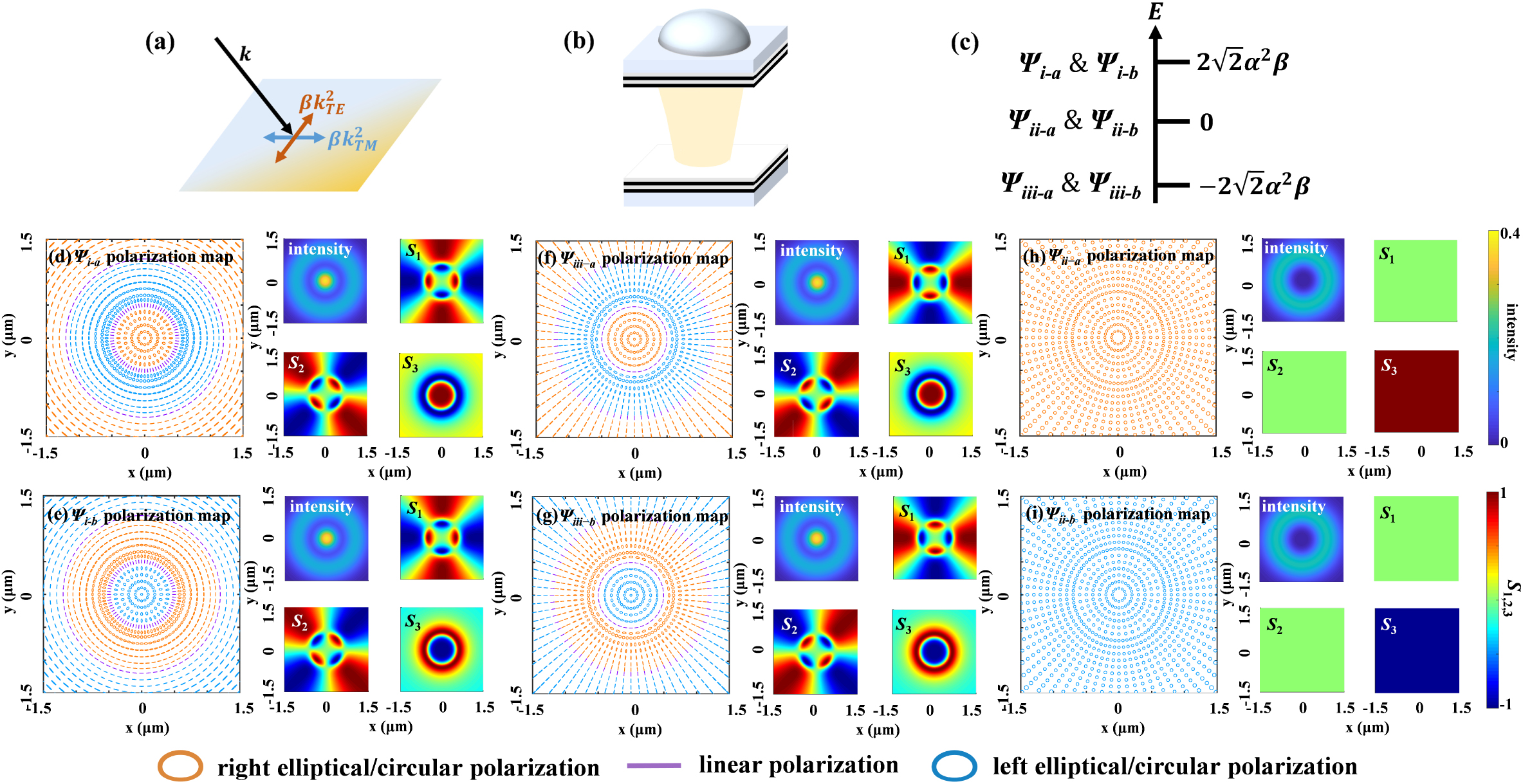
Fig. 1. Polarization textures of the eigenstates of the second excited manifold. (a) Schematic of the TE-TM splitting characterized by β. (b) Sketch of an open-access microcavity; the concave-planar mirror configuration provides the confined potential V. (c) Energy levels of the eigenstates under the effect of TE-TM splitting. α is the parameter determining mode size. (d)–(i) Left panels, polarization textures of each eigenstate which is instructed in the main text; right panels, the four small graphs representing the intensity distribution, Stokes components S1, S2, and S3. The states presented in (d) and (e), (f) and (g), (h) and (i) are all twofold degenerate in energy. The following parameters are used: α=1.54  μm−1, β=0.06  meV·μm2.

Fig. 2. Optical skyrmions with lifting and keeping the mode degeneracy. (a) Left panel, polarization textures of the linear combination of degenerate skyrmion-like states with J=±1 at zero phase difference; right panels, the four small graphs represent the intensity distribution, Stokes components S1, S2, and S3. (b) Polarization degree S0 of the incoherent superposition of the two degenerate skyrmion-like states.

Fig. 3. Non-Hermitian control of the optical skyrmions. (a) Real and (b) imaginary parts of the eigenvalues as a function of the circular gain and loss ρ. (c) and (d) are, respectively, the same as (a) and (b) except that ρ is enveloped by Gaussian-like spatial distribution with the size parameter σ=3.08  μm−1. The following parameters are used: α=1.54  μm−1, β=0.06  meV·μm2.

Fig. 4. Evolution of the polarization textures of Ψi−a in Fig. 3 under non-Hermitian manipulation. (a)–(c) intuitively show the change of polarized state with the increase of ρ with spatially uniform gain and loss corresponding to Figs. 3(a) and 3(b). (d) Poincaré sphere representation of polarization texture evolution. Coordinates S1, S2, and S3 are three components of Stokes vectors. Point P denotes the polarization state at the red spatial point shown in (a)–(c), which locates at positions P1, P2, and P3 when (a) ρ=0, (b) ρ=0.40167 (at EP), and (c) ρ=0.5, respectively. (e) Polarization texture of Ψi−a at the EP with Gaussian-enveloped gain and loss. The four small graphs on the right panels of (a)–(c) and (e) represent the intensity distribution, Stokes components S1, S2, and S3, respectively, while the left panels represent the polarization texture drawings. The following parameters are used: α=1.54  μm−1, β=0.06  meV·μm2.

Fig. 5. Non-Hermitian control of the second manifold states with elliptical asymmetry of the photonic potential. (a) Real and (b) imaginary parts of the eigenvalues as a function of the circular gain and loss ρ with Gaussian-like envelope. The enlarged parts of the bifurcation of the real (imaginary) part are shown in (a-1) and (a-2) [(b-1) and (b-2)]. The following parameters are used: α=1.54  μm−1, β=0.06  meV·μm2, and δ=0.15.

Fig. 6. Evolution of the polarization textures of Ψ1 in Fig. 5 under the non-Hermitian manipulation. The left panels of (a)–(f) intuitively show the change of polarized state with the increase of ρ. The right panels are the four small graphs representing the intensity distribution, Stokes components S1, S2, and S3, respectively. The values of S3 are uniform in (a)–(e). In (a)–(c) S3=0, while in (d) S3=0.65 and (e) S3=0.7.

Fig. 7. Spatial distribution of the 3D vector n=(nx,ny,nz). (a)–(c) correspond to the eigenstates in Figs. 1(d), 4(b), and 1(f) of the main text, within the region of x2+y2≤0.65  μm. Each group contains a 3D map of the vector n and the 2D colored maps of nz [i.e., cos β(r)] and arctan(ny/nx) [i.e., α(θ)]. The range of arctangent values is set from –π to π to cover the 2π range of the angle α of the Poincaré sphere. Note that the parts of the graphs exceeding the range of x2+y2≤0.65  μm are out of the skyrmion structure and, therefore, do not represent proper physical meaning, which is just an extension out of the proper range to fit the square-shaped graph boundary.

Table 1. Total Angular Momentum J of the Second Excited Manifold LG Modes^a