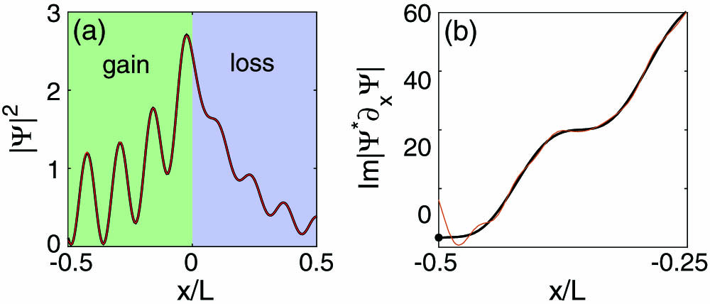
Fig. 1. (a) Total wave function and (b) its flux depicted by black thick lines for a half-gain-half-loss microcavity with light incident from the left. The wave vector k=12/L and refractive indices n1=n2*=2−0.2i are used. The expansion in Eq. (14) with 50 CF states is plotted by the red thin lines as a comparison, which can barely be distinguished from the black line in (a) but shows a significant deviation near the left boundary in (b). The black dot in (b) shows the analytical result at x=−L/2 given by Eq. (18).

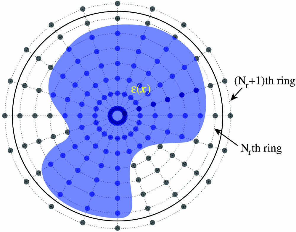
Fig. 2. Schematic of an optical microcavity (shaded area) and the circular LSS (solid line) in 2D. The finite-difference grid is indicated by the dots and dashed lines.

Fig. 3. Resonances of a microdisk cavity with a uniform index n=1.5. The crosses are the analytical results given by Eq. (52), and the circles are the poles of the S matrix constructed using Eq. (28).

Fig. 4. (a) Spontaneous symmetry breaking of S-matrix eigenvalues sn in a microdisk cavity with PT and RT symmetries. Its refractive index is given by n(x)=1.5+0.4 sin θ, the imaginary part of which is shown schematically by the inset in (b). (b) A real-valued eigenvector of S at kR=4 in the PT- and RT-symmetric phase. The blue (pink) bars show symmetric and antisymmetric components with opposite m’s. The corresponding wave function is shown in (d), where the cavity boundary is marked by the white circle. The wave function of a scattering eigenstate in the broken-symmetry phase at kR=4 is shown in (c) as a comparison.

Fig. 5. Resonant modes corresponding to the scattering eigenstates in Figs. 4(c) and 4(d).