
Yanan Han, Shuiying Xiang, Yang Wang, Yuanting Ma, Bo Wang, Aijun Wen, Yue Hao. Generation of multi-channel chaotic signals with time delay signature concealment and ultrafast photonic decision making based on a globally-coupled semiconductor laser network[J]. Photonics Research, 2020, 8(11): 1792
- Photonics Research
- Vol. 8, Issue 11, 1792 (2020)
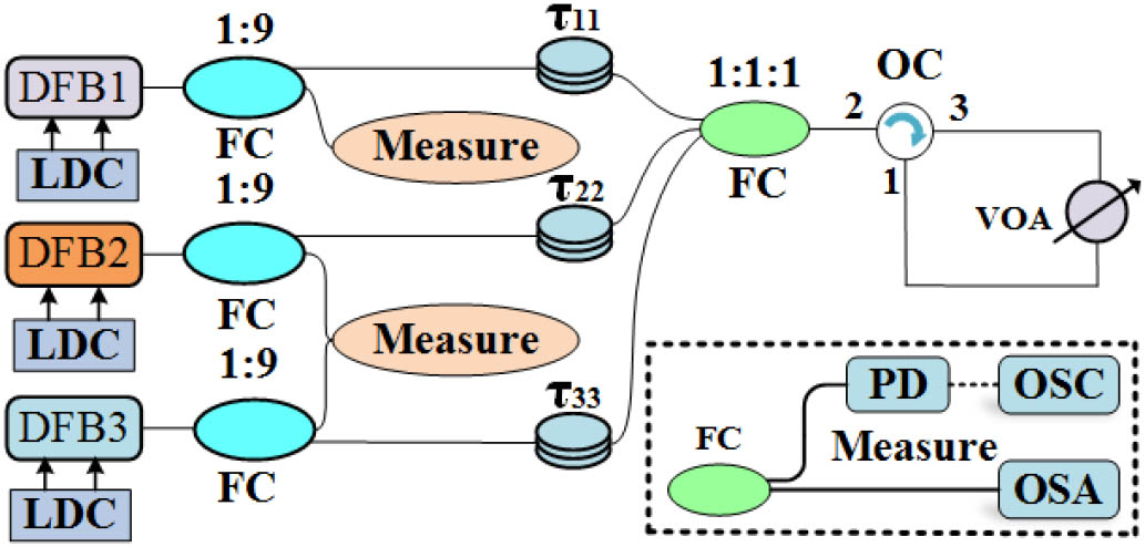
Fig. 1. Experimental setup of three globally coupled SLs. DFB1, DFB2, DFB3, three distributed feedback lasers; LDC; laser diode controller; FC, fiber coupler; OC, optical circulator; VOA, variable optical attenuator; τ 11 , τ 22 , τ 33
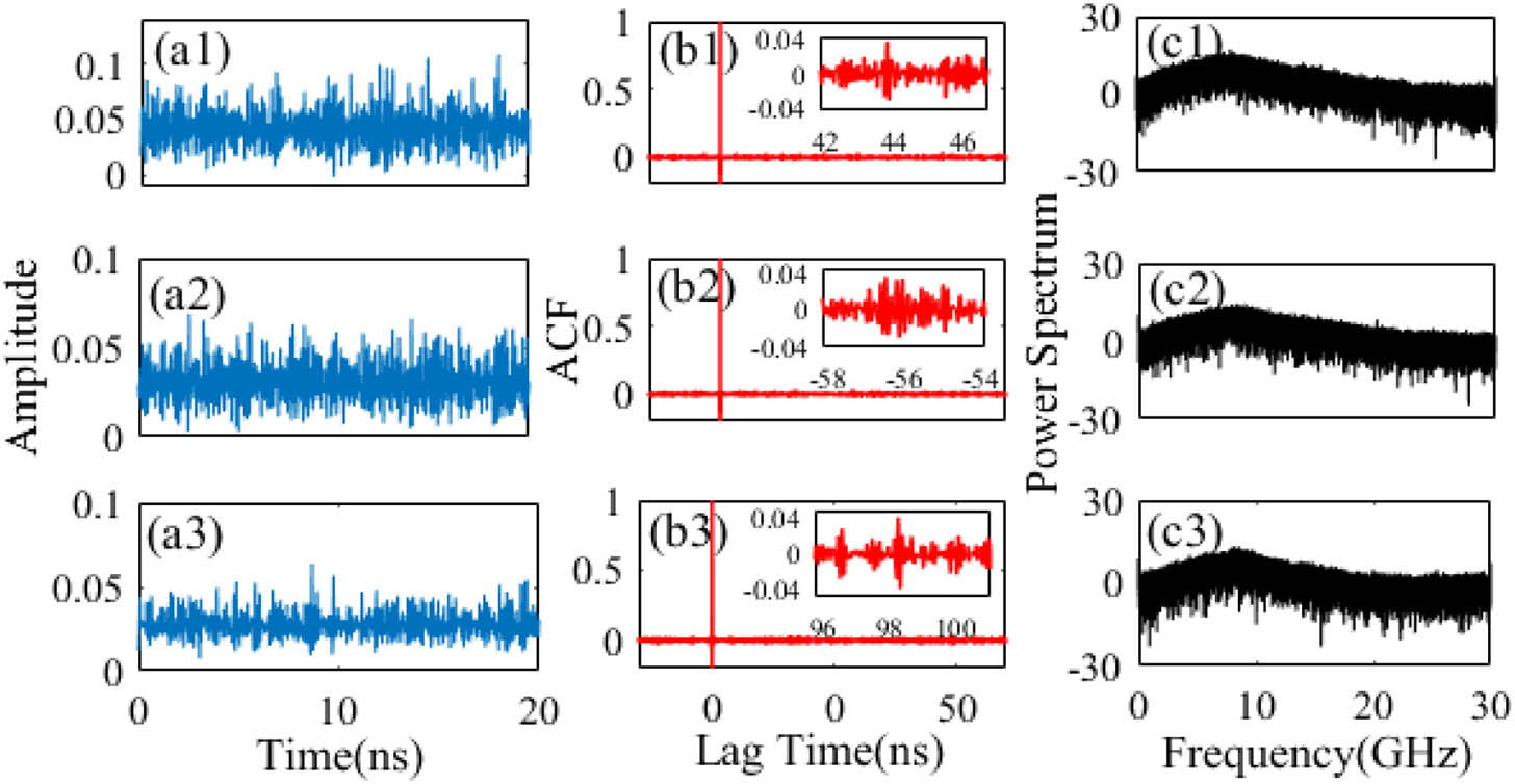
Fig. 2. (a1)–(a3) The chaotic time series from the three DFB lasers; (b1)–(b3) the ACFs; (c1)–(c3) the power spectra. The attenuation is 9 dB, I 1 , I 2 , I 3 = 28.34 , 24.5 , 26.6 mA T 1 , T 2 , T 3 = 27.75 , 15.5 , 18 ° C
Fig. 3. (a) ρ m ρ m I 2
Fig. 4. (a1)–(a3) Time series of signals at states I, II, and III, respectively; (b1)–(b3) the corresponding power spectrum.
Fig. 5. (a1)–(a3) The chaotic time series from the three SLs; (b1)–(b3) the ACFs, (c1)–(c3) the power spectra. The parameters are: I m = 20 , 22.5 , 20 mA k r m = 11.7 , 16.7 , 11.7 ns − 1 τ m m = 2 , 2.02 , 2.04 ns m = 1 , 2 , 3
Fig. 6. (a1)–(a3) The two-dimensional map of ρ m k r 2 I 2 I 1 = I 3 , I 2 = I 1 + 2.5 mA k r 1 = k r 3 , k r 2 = k r 1 + 5 ns − 1 τ m m = 2 , 2.02 , 2.04 ns
Fig. 7. TDS concealment with different time delays. I 1 = I 3 I 2 = I 1 − 1 mA k r m = 12,10 , 12 ns − 1 τ m m = 3 , 3.02 , 3.06 ns , m = 1 , 2 , 3 I 2 = I 1 − 1 mA k r m = 12,11 , 12 ns − 1 τ m m = 3 , 3.1 , 3.2 ns I 2 = I 1 − 2 mA , k r m = 13.3 , 12.3 , 13.3 ns − 1 τ m m = 4 , 4.07 , 4.13 ns ρ m τ 11 τ 22 = τ 11 + 0.3 ns τ 33 = τ 11 + 0.7 ns I m = 21,19 , 21 mA k r m = 12,10 , 12 ns − 1 m = 1 , 2 , 3
Fig. 8. Architecture for the eight-armed bandit problem processed in parallel based on triple-channel chaos.
Fig. 9. Evolution of CDR for the triple-channel signals with different correlations and for the one-channel scheme. The vertical bars indicate the standard deviation around the mean value for three sets of simulated signals. P = [ 0.2,0.2,0.8,0.2,0.2,0.2,0.2,0.2 ]
Fig. 10. CC with different sampling intervals for the one-channel and triple-channel schemes, respectively. The vertical bars indicate the standard deviation around the mean value for eight sets of simulated signals. P = [ 0.8,0.2,0.2,0.2,0.2,0.2,0.2,0.2 ]
Fig. 11. (a), (b) CC and ρ m ρ m < 0.2 ρ m > 0.3 P = [ 0.3,0.2,0.8,0.1,0.2,0.3,0.5,0.4 ]
Fig. 12. CC as a function of bias current, for a comparison of the triple-channel scheme (red solid line), the previously investigated parallel scheme (blue dotted line), and the one-channel scheme (black solid line). The vertical bars indicate the standard deviation around the mean value for three runs. P = [ 0.3,0.2,0.8,0.1,0.2,0.3,0.5,0.4 ]
Fig. 13. (a) Evolution of the CDR for different distributions of reward probability in a changing environment. P 1 = [ 0.8, 0.2,0.2,0.2,0.2,0.2,0.2,0.2 ] P 2 = [ 0.7,0.2,0.3,0.2,0.2,0.2,0.2,0.2 ] P 2.
Fig. 14. Evolution of the averaged CDR with randomly selected signals for eight-armed and 16-armed bandit problems. P = [ 0.3,0.2,0.8,0.1,0.2,0.3,0.5,0.4 ] P = [ 0.3,0.2,0.8,0.1,0.2,0.5, 0.2,0.2,0.2,0.3,0.3,0.4,0.5,0.1,0.1,0.2 ]

Set citation alerts for the article
Please enter your email address
© Copyright 2018-2021 | Chinese Laser Press. All Rights Reserved 沪ICP备15018463号-20