Yanan Han, Shuiying Xiang, Yang Wang, Yuanting Ma, Bo Wang, Aijun Wen, Yue Hao, "Generation of multi-channel chaotic signals with time delay signature concealment and ultrafast photonic decision making based on a globally-coupled semiconductor laser network," Photonics Res. 8, 1792 (2020)
Copy Citation Text
We propose and demonstrate experimentally and numerically a network of three globally coupled semiconductor lasers (SLs) that generate triple-channel chaotic signals with time delayed signature (TDS) concealment. The effects of the coupling strength and bias current on the concealment of the TDS are investigated. The generated chaotic signals are further applied to reinforcement learning, and a parallel scheme is proposed to solve the multiarmed bandit (MAB) problem. The influences of mutual correlation between signals from different channels, the sampling interval of signals, and the TDS concealment on the performance of decision making are analyzed. Comparisons between the proposed scheme and two existing schemes show that, with a simplified algorithm, the proposed scheme can perform as well as the previous schemes or even better. Moreover, we also consider the robustness of decision making performance against a dynamically changing environment and verify the scalability for MAB problems with different sizes. This proposed globally coupled SL network for a multi-channel chaotic source is simple in structure and easy to implement. The attempt to solve the MAB problem in parallel can provide potential values in the realm of the application of ultrafast photonics intelligence.
1. INTRODUCTION
Since its advent, the laser has been applied in many fields due to the advantages of rapid response and rich dynamics [1]. For example, it is used in high-speed random bit generators [2,3], optical secure communication, and secret key distribution that requires synchronized chaotic signals [4–7]. Recently, photonic technologies have also been developed as efficient ways of solving some conventional problems in the area of artificial intelligence (AI) calculation such as reservoir computing [8,9], reinforcement learning [10–12], and brain-inspired photonic neuromorphic computing [13–16].
The security of information transmission has always been a focus of attention. In optical communication systems, chaotic signals can be generated by means of delayed optical feedback, optical injection, and other external disturbances [17–22]. However, a time delay signature (TDS) can be introduced (typically by external cavity feedback) and cause internal periodicity of chaotic oscillations [23,24]. This feature can be analyzed by methods like permutation entropy (PE), delayed mutual information, autocorrelation functions (ACF), etc., and utilized for reconstruction of chaotic systems [25–29], which seriously threaten the security of communication. Many methods have been reported to complicate and suppress the TDS. For example, Lee et al. first proposed to complicate the TDS in a semiconductor laser (SL) subject to double optical feedback [30], and the result was experimentally demonstrated later by Wu et al. [31]. We also numerically achieved the suppression of TDS in a mutually coupled ring network with heterogeneous time delays [32]. Very recently, Jiang et al. proposed a new scheme for the generation of wideband laser chaos with excellent TDS suppression by using parallel-coupling ring resonators as reflector [33].
As one of the fundamental problems in reinforcement learning, adequate decision making in a dynamically changing environment is also required in frequency and channel assignments in communication networks [12,34,35]. The multiarmed bandit (MAB) problem is one of the most important issues in decision making. One remarkable method to solve the MAB problem was proposed by Kim et al., called the tug-of-war (TOW) method, which was inspired by the unicellular amoeba of true slime mold [36,37]. In recent years, several works on ultrafast decision making have been reported based on the TOW method [38–41]. In our previous work, we have already proposed to solve a four-armed bandit problem in parallel by sampling dual-channel TDS-concealed chaotic signals simultaneously and found it works more efficiently [42]. However, the threshold value (TV) for each channel is set and adjusted dependently; therefore, the scheme is not completely parallel.
Sign up for Photonics Research TOC. Get the latest issue of Photonics Research delivered right to you!Sign up now
In this paper, we propose a scheme for the generation of laser chaos with TDS concealment and demonstrate its application in reinforcement learning. Our contribution includes three aspects. First, the new proposed scheme for the generation of complex laser chaos is simple in structure and easy to implement. Second, we propose a scheme to solve the MAB problem in parallel via using the generated laser chaos and verify its scalability and adaptability. Third, in order to solve the MAB problem in parallel, we propose a modified strategy and demonstrate its effectiveness.
2. SYSTEM MODEL AND RESULTS
A. Experimental Setup
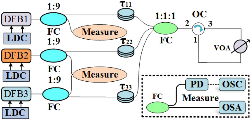
The experimental setup of three globally coupled SLs is presented in Fig. 1. Here, three distributed feedback (DFB) lasers are driven by laser diode controllers (LDCs) to control the current and temperature of the SLs. The wavelengths of free-running DFB lasers are precisely matched by adjusting the current and temperature. In this setup, the optical output from each DFB laser is divided into two parts through a 10:90 fiber coupler (FC). The smaller part is sent to the measure module, where the optical signal can be detected by a high-speed photodiode (PD, HP11982A, 15 GHz) and analyzed by a real-time oscilloscope (OSC) with 8-bit analog-to-digital converter (Keysight DSOV334A, 33 GHz, 80 GS/s), or directly sent to an optical spectrum analyzer (OSA, AndoAQ6317). The rest of the parts are combined into one with an FC through fiber jumpers with different lengths, then pass through a variable optical attenuator (VOA), and feed back to all the three DFB lasers via an optical circulator (OC). Thus, the coupling strength and feedback strength can be adjusted simultaneously by the VOA. For simplicity, they are referred to as coupling strength in the following.
The ACF is one of the effective methods for identifying the TDS of the measured chaotic signals [29,32], as defined in Eq. (1), where is the ACF value of the chaotic time series at time lag , measured from DFBm (m = 1, 2, 3). means time average. The TDS concealment can be reflected by the most pronounced residual peak, denoted as ,in the ACF. Better TDS concealment is indicated by a lower value of [32].
To identify the TDS of DFB1, we turn off DFB2 and DFB3, and calculate the ACF of the output intensity; the round-trip feedback time delay of DFB1 is indicated by the location of in the ACF. By this method, the feedback time delays for DFB1, DFB2, and DFB3 are determined to be 97.4, 97.53, and 97.38 ns, respectively. Note that the time delay values are close, introduced by slightly different propagation paths, and need not be precisely adjusted by the variable optical delay line (VODL). The wavelengths of free-running DFB lasers are precisely set as 1552.250, 1552.265, and 1552.255 nm, respectively, by carefully adjusting the current and temperature.
Figure 2 shows the measured chaotic time series from the three DFB lasers, the calculated ACF as a function of , as well as the power spectrum. The chaotic dynamics of the three SLs can be revealed by the time series shown in Figs. 2(a1)–2(a3) and the power spectrum in Figs. 2(c1)–2(c3). As can be seen in Figs. 2(b1)–2(b3), no pronounced peaks can be found in the ACFs except for that at time lag 0, which means the TDS is greatly concealed in all three channels.
Figure 2.(a1)–(a3) The chaotic time series from the three DFB lasers; (b1)–(b3) the ACFs; (c1)–(c3) the power spectra. The attenuation is 9 dB, , .
Then, in order to illustrate the effect of coupling strength on TDS concealment, the as a function of attenuation is presented in Fig. 3(a). Region I (III) indicates that all three DFB lasers are in a quasi-periodic state (chaotic state). Region II represents the transition region where the states of the three DFB lasers can be quasi-periodic, weakly chaotic, and chaotic, but not identical. Examples of the time series and the power spectrum of signals in each state are shown in Fig. 4. It can be seen that is less than 0.1 when the attenuation is larger than 5.0 dB and increases with the decrease of attenuation, indicating that better TDS concealment can be achieved when the attenuation is large, namely, when the coupling strength is relatively small. The influence of bias currents on the TDS concealment is further investigated, as shown in Fig. 3(b). Here, the bias currents of the three DFBs are adjusted at the same time, and we simply present as a function of (which varies from 18.6 to 34.6 mA). It can be seen that is less than 0.1 when , indicating that low TDS can be obtained in that region. However, when , the values are larger than 0.1 and get larger with the increase of , indicating reduced concealment of TDS for all three DFB lasers.
Figure 3.(a) as a function of attenuation; (b) as a function of .
In addition, we also numerically verified the concealment of TDS in the proposed scheme. To model the dynamics of the three DFB lasers, the well-known Lang–Kobayashi equations are adopted, which describe the slowly varying complex electric-field and the carrier density in the active region [31,32]. The rate equations of our scheme can be written as where denotes the three SLs. is the linewidth enhancement factor [32,43], is the differential gain coefficient, is the nonlinear gain saturation coefficient, and and stand for the photon lifetime and the carrier lifetime, respectively. is the transparency carrier number. The variable represents the bias current and describes the coupling strength. The coupling time delay from to can be calculated from the feedback time delay by .
In Fig. 5, we present the time series, the ACF, and the power spectrum of the numerical results as in Fig. 2. The results show that the TDS can be concealed in such a scheme if the parameters are properly selected. Note that the mismatch of parameters is important to improve the concealment of the TDS. When the currents are the same for the three SLs, the region in which the TDS is concealed is quite narrow. To find a proper bias current, we can fix the currents of two SLs and change the other. In this way, we find that a current mismatch of 0.5–3.5 mA allows better TDS concealment in all three SLs. We choose a mismatch of 2.5 mA.
Figure 5.(a1)–(a3) The chaotic time series from the three SLs; (b1)–(b3) the ACFs, (c1)–(c3) the power spectra. The parameters are: ; ; ; .
For a further exploration of the parameters’ scope in which the TDS can be better suppressed, we show in Figs. 6(a1)–6(a3) the two-dimensional map of for the three SLs as functions of the coupling strength and bias current of (for simplicity). The parameter region for is considered to have better TDS concealment and is marked by a white dotted line [32]. It can be seen that the evolution patterns for three are similar, and the parameters for low TDS are mainly in the diagonal region, meaning that concealment is affected by both the current and the strength. The PE is also calculated as an indicator of the dynamical state of SLs [44] and is presented in Figs. 6(b1)–6(b3). The dynamics of the SL is in chaotic oscillation when the PE value is larger than 0.99, marked by a black dotted line. As PE decreases, the dynamics goes through chaos to weak chaos and finally enters quasi-periodic oscillation.
Figure 6.(a1)–(a3) The two-dimensional map of as functions of the coupling strength and bias current of DFB1, DFB2, and DFB3, respectively; (b1)–(b3) the PE of DFB1, DFB2, and DFB3, respectively. ; ; .
Moreover, time delay is also an important factor that affects the dynamics of a system, and different time delays may cause different sensitivities to parameter mismatches. Hence, it is necessary to consider different coupling delays in the investigation of TDS concealment. Figures 7(a)–7(c) depict the as a function of with three different cases of time delay. We can see that in all three cases, the TDS can be concealed with properly selected parameters. Typically, we find that for a larger time delay, stronger coupling strength is required to achieve better TDS concealment. In Fig. 7(d), we further show the as a function of for all three SLs. It can be seen that for fixed current and coupling strength, the values of remain relatively small as varies from 1 to 8 ns. The results indicate that in this scheme, the TDS concealment can be achieved with different time delays.
Figure 7.TDS concealment with different time delays. . (a) , , ; (b) , , , (c) ; , (d) as a function of . , , , , .
In this section, we utilize the triple-channel chaotic signals generated from the above scheme to solve an eight-armed bandit problem in parallel. By choosing one of eight slot machines, there is a chance of getting a reward. The reward probabilities are different and unknown to users [40]. Users need to explore the slot machines to find the one that has the highest reward probability, which we call the target machine. Due to the trade-off known as the exploration-exploitation dilemma [40,41], the exploration needs to be effective so that the target machine can be found as quickly as possible and without the risk of missing it.
A. Scheme of Solving MAB Problem in Parallel
For an -armed bandit problem, where with being a natural number, -bit binary number can be used to distinguish the slot machines [41]. When (), the eight slot machines can be encoded by . Figure 8 gives the schematic diagram for solving the eight-armed bandit problem in parallel. We propose a modified strategy for the implementation of the parallel scheme, in which the triple-channel chaotic signals are simultaneously sampled and are, respectively, compared with the threshold values of each channel. Before sampling, the signals are standardized and normalized. A decision is made according to the comparison result, that is, if , , else . To be specific, suppose that the triple-channel chaotic signals sampled at are ; then they are compared with the threshold values , respectively. If , the most significant bit is determined as ; if , the second-most significant bit is ; if , the last-significant bit is . Therefore, the slot machine 1, marked by , is chosen. If a reward is given by choosing slot machine 1, then the threshold values are adjusted so that the same decision is more likely to be made in the next cycle. Otherwise, if no reward is yielded, the threshold values are adjusted to reduce the probability of making the same choice the next time.
Figure 8.Architecture for the eight-armed bandit problem processed in parallel based on triple-channel chaos.
The threshold values of the three channels are independently updated according to , where is the threshold adjuster and takes the integer value from . is a constant integer. Here we set . is a constant factor to limit the range of . The threshold values are adjusted as follows.
If the selected slot machine yields a reward at , the TV value is updated at by
If the selected slot machine yields no reward at , the TV value is updated at by where the increment parameter is fixed unity [41], is a constant memory parameter, is determined based on the history of getting rewards, and is given by [42]
is the total number of times selecting . is the number of times that one gets a reward by selecting . The initial value of is set to 0. Note that for an -armed bandit problem where , it only requires -channel signals and -threshold values, which greatly simplifies the implementation compared with the previous method that requires threshold values [41,42].
C. Results and Discussion
To describe the decision-making performance, we define convergence cycle (CC) as the number of the first cycle that reaches a correct decision rate (CDR) of 0.9, where is the ratio of the times of getting a reward and the total number of selections. In practice, the average accuracy rate is often adopted to describe a short-time behavior, as the environment is always changing [45]. Here, the CDR is averaged over 400 repeated runs.
Due to the parallel structure of our scheme, the cross correlation among the triple-channel chaotic signals should be taken into account. The cross-correlation function is introduced as [5] where is the cross-correlation coefficient of signals from and at time lag . The zero lag correlation () can be accurately controlled by shifting the signals in the time domain.
Three channels of zero-lag synchronized chaotic signals may cause an ultrafast convergence when the target is encoded as [0,0,0], making it nearly impossible to recognize the target machine [0,1,0]. For simplicity, to investigate the impact of correlation on the performance of decision making, we only consider the effect of , and the values of and are kept close to 0. In Fig. 9, we show the CC as a function of for three sets of numerically generated signals with different correlations, where . Additionally, the result of the one-channel scheme is also calculated for a brief comparison. Here, the distribution of reward probability is . It can be seen that as the cross correlation decreases, the CC of the triple-channel scheme is smaller and becomes less than that of the one-channel scheme when . This critical value may change with different distributions of reward probability and with different signals. The result shows, obviously, that the performance of the triple-channel scheme could outstrip the one-channel scheme when the correlation of the signals is quite low (which is easy to realize for chaos signals). Therefore, in order to reduce the impact of correlation among the triple-channel signals, we properly shift each set of signals in the time domain so that their cross-correlation coefficient at zero-time lag is around 0. Here, the time lags for the three signals to avoid the cross correlation are 0, 1, and 2 ns, respectively.
Figure 9.Evolution of CDR for the triple-channel signals with different correlations and for the one-channel scheme. The vertical bars indicate the standard deviation around the mean value for three sets of simulated signals. .
Next, we compare the decision-making performance of the one-channel scheme and the triple-channel scheme by calculating the CC with different sampling intervals. The results are illustrated in Fig. 10. It can be seen that for both schemes, it converges quickly when the sampling interval is as small as 10 ps, which requires the highest sampling rate that is currently available, but slows down with the increase of sampling interval. Hence, we choose a sampling rate of 10 ps in the following. Also note that the CC value of the triple-channel scheme is statistically lower and grows more slowly than that of the one-channel scheme, which means that in the proposed scheme, it can converge more quickly to the desired accuracy, and the performance is relatively stable against the variation of sampling interval. Note that in Fig. 10 and the following, the CC value of the one-channel scheme is the average of the results of three channel signals.
Figure 10.CC with different sampling intervals for the one-channel and triple-channel schemes, respectively. The vertical bars indicate the standard deviation around the mean value for eight sets of simulated signals. .
Then the experimentally generated signals with varying attenuation are utilized to investigate the influence of TDS on the decision-making performance. The CC as a function of attenuation is presented in Fig. 11(a), and in Fig. 11(b) we show the result of for ease of comparison. The laser dynamics is clarified, as in Fig. 3. It is obvious that when , especially when it reaches about 0.6, the cycle to reach a CDR of 0.9 is quite large. When , the change of CC is not directly linked with , but overall, a smaller CC appears with lower . Note that the signals are normalized during preprocessing, so it is not the amplitude of the signals but the characteristics that affect the result. In addition, for a deeper understanding of the influence of TDS suppression on the decision-making performance, we statistically investigate the evolution of CDR using numerical signals with different TDS concealments, where the value of is controlled by slightly changing the bias current, the coupling strength, or the coupling delay of the three SLs. In Fig. 11(c), we show the CDR as a function of the learning cycles using 11 sets of signals with and , respectively. It can be seen that there exist signals with larger that still converge more quickly than those with lower , showing that the decision-making performance does not entirely depend on the suppression of TDS. However, on the whole, it converges faster for signals with lower in a decision-making problem, which indicates that the concealment of TDS can be helpful for better decision-making performance.
Figure 11.(a), (b) CC and as functions of attenuation; (c) CDR as a function of learning cycles. The vertical bars indicate the standard deviation around the mean value for 11 sets of signals with and , respectively. The sampling interval is 10 ps. .
Next, we compare the decision-making performance of the one-channel scheme, the previously proposed parallel scheme [42], and the triple-channel scheme by calculating the CC, where experimentally generated signals with different bias currents are adopted. The results are illustrated in Fig. 12. Triple-channel1 and Triple-channel2 represent the new scheme and the previously proposed scheme, respectively. Three channels of signals are used to solve the eight-armed bandit problem. However, in the Triple-channel2 scheme, the adopted algorithm for threshold adjustment is the same as in the one-channel scheme. It can be seen that for both the triple-channel schemes, the CC is quite stable against the variation of bias current, and the performance is quite similar, whereas for the one-channel scheme, it takes more cycles to reach the desired CDR, and the CC value fluctuates more obviously with the change of bias current, indicating that the one-channel scheme may be more sensitive to the dynamics of signals.
Figure 12.CC as a function of bias current, for a comparison of the triple-channel scheme (red solid line), the previously investigated parallel scheme (blue dotted line), and the one-channel scheme (black solid line). The vertical bars indicate the standard deviation around the mean value for three runs. .
In addition, it is necessary to make decisions accurately in a dynamically changing environment, where the slot machine with the highest reward probability may change with time. Figure 13(a) illustrates the evolution of the CDR in a changing environment. We suppose that the target machine changes from slot machine 1 to 3 at the 600th cycle, and slot machines with different probability distributions are considered for comparison. It can be seen that after the sudden change of the target machine, the CDR drops to zero, and then increases rapidly. Meanwhile, one can see that it takes longer time to reach a CDR of 0.9 for P2 than that for P1, because the former has less difference in the distribution of reward probability [12,46]. To further reveal the underlying process of the reinforcement learning, the adaption of the threshold values during the 1200 cycles is presented in Fig. 13(b). In the first 600 cycles where the target slot machine is encoded as [0,0,0], the threshold values , , and all increase until they eventually fluctuate around a maximum value of 0.5. Hence, the chaotic signals are more likely to be lower than the threshold values , and the three significant bits [D1,D2,D3] are more likely to be determined as [0,0,0]. When the target machine changes to [0,1,0], after temporary fluctuation around 0, the values of and return to about 0.5. The value of is reduced to about , which makes it more possible for to be larger than , and further results in an increase in the likelihood of choosing the slot machine [0,1,0].
Figure 13.(a) Evolution of the CDR for different distributions of reward probability in a changing environment. , . (b) Threshold value adaption for P2.
Scalability is also very important for a decision-making scheme. Due to the chaotic dynamics of signals, it can be assumed that arbitrarily selected -channel chaotic signals that are generated from the scheme as in Fig. 1 can be utilized to solve the -armed bandit problem successfully. To demonstrate this, three channels of experimentally generated signals with varying bias current are randomly selected to solve the eight-armed bandit problem. The evolution of the CDR is presented in Fig. 14, denoted by a red solid line, and the vertical bars indicate the standard deviation around the mean value for 10 different selections. It can be seen that the average CDR is about 330, similar to the result in Fig. 12. Meanwhile, eight different selections of four-channel signals are successfully used to solve a 16-armed bandit problem. The evolution of the CDR is also shown in Fig. 14, represented by the dashed blue line. These results show that random combination of chaotic signals is capable of solving the MAB problem efficiently, and the scalability of our scheme to larger decision problems is verified.
Figure 14.Evolution of the averaged CDR with randomly selected signals for eight-armed and 16-armed bandit problems. , and , respectively.
In conclusion, we propose a simple scheme of achieving triple-channel chaotic signals with TDS concealment and demonstrate it via experiment and numerical analysis. The parameters’ range that contributes to better TDS concealment is explored by systematically changing the bias current and the coupling strength. Moreover, we utilize the generated triple-channel chaotic signals and a modified strategy for the realization of an eight-armed bandit problem in parallel; the influences of the signal correlation between each channel, the TDS concealment, and the sampling interval on the performance of decision making are investigated. In the proposed decision-making scheme, the simplified algorithm compared with the one-channel scheme and the previously studied parallel scheme makes it easier for implementation. However, it can perform even better given that the mutual-correlation is relatively low. Moreover, it has stabler performance for different sampling rates than the one-channel scheme. The proposed system is scalable to varying size of MAB problems and is adaptable in changing environments. This work may be helpful for potential applications in the ultrafast processing of AI.
References
[1] J. Ohtsubo. Semiconductor Lasers: Stability, Instability and Chaos(2012).
Yanan Han, Shuiying Xiang, Yang Wang, Yuanting Ma, Bo Wang, Aijun Wen, Yue Hao, "Generation of multi-channel chaotic signals with time delay signature concealment and ultrafast photonic decision making based on a globally-coupled semiconductor laser network," Photonics Res. 8, 1792 (2020)