• Photonics Research
  • Vol. 10, Issue 7, 1712 (2022)
Vassily Kornienko*, David Andersson, Mehdi Stiti, Jonas Ravelid, Simon Ek, Andreas Ehn, Edouard Berrocal, and Elias Kristensson
Author Affiliations
  • Division of Combustion Physics, Department of Physics, Lund University, Lund, Sweden
  • show less
    DOI: 10.1364/PRJ.451108 Cite this Article Set citation alerts
    Vassily Kornienko, David Andersson, Mehdi Stiti, Jonas Ravelid, Simon Ek, Andreas Ehn, Edouard Berrocal, Elias Kristensson. Simultaneous multiple time scale imaging for kHz–MHz high-speed accelerometry[J]. Photonics Research, 2022, 10(7): 1712 Copy Citation Text show less
    System capable of monitoring microscopic MHz dynamics with kHz technology. (a) The light from each nanosecond pulsed laser source, triggered w.r.t the high-speed camera, is spatially modulated with Ronchi gratings (20 lp/mm) and combined into a pulse train incident on the sample. The imaged event is then relayed to the high-speed camera via a microscopy configuration. Due to the laser pulses’ temporal separation [inset of (a)] the event of interest will be illuminated at three distinct times within a single camera exposure. (b) Each high-speed camera image consists of three superimposed spatially modulated images of which an example is framed in red. Its Fourier transform depicts distinct peaks, within which the individual pulse information is contained. Performing a spatial lock-in followed by low-pass filtering on the peaks extracts said information. (c) Carrying out this process (including background correction) on each high-speed camera image results in a video sequence where bursts of three images (FRAME triplets) are taken at a repetition rate set by the camera, allowing, e.g., the extraction of 2D accelerometry data from each camera image. The complete video of (c) is included as Visualization 4.
    Fig. 1. System capable of monitoring microscopic MHz dynamics with kHz technology. (a) The light from each nanosecond pulsed laser source, triggered w.r.t the high-speed camera, is spatially modulated with Ronchi gratings (20 lp/mm) and combined into a pulse train incident on the sample. The imaged event is then relayed to the high-speed camera via a microscopy configuration. Due to the laser pulses’ temporal separation [inset of (a)] the event of interest will be illuminated at three distinct times within a single camera exposure. (b) Each high-speed camera image consists of three superimposed spatially modulated images of which an example is framed in red. Its Fourier transform depicts distinct peaks, within which the individual pulse information is contained. Performing a spatial lock-in followed by low-pass filtering on the peaks extracts said information. (c) Carrying out this process (including background correction) on each high-speed camera image results in a video sequence where bursts of three images (FRAME triplets) are taken at a repetition rate set by the camera, allowing, e.g., the extraction of 2D accelerometry data from each camera image. The complete video of (c) is included as Visualization 4.
    Microscopic imaging of transient fluid dynamics at high speed. (a) Imaging the spray injection event at a camera speed of 21 kHz and a shutter time of 12 μs within which three pulses, with constant inter-pulse time (250 kHz FRAME triplet), are recorded. (b) Non-linear temporal triggering where the first two pulses arrive at the sample with an inter-pulse time of 20 μs (50 kHz), while the last two are incident with an inter-pulse time of 2 μs (500 kHz). At the beginning of the event, 50 kHz suffices to track the fluid’s evolution within the camera exposure, while already at 95 μs ASOI, higher speeds are necessary. The zoom-ins of the USAF 1951 resolution target correspond to the resolution limits in x and y of the current optical configuration. (c) Imaging the injection event with 21 kHz camera speed and 10 MHz FRAME triplet (100 ns inter-pulse time) while retaining the image spatial resolution of (b). See Visualization 1, Visualization 2, Visualization 5, and Visualization 6 for videos of the entire events.
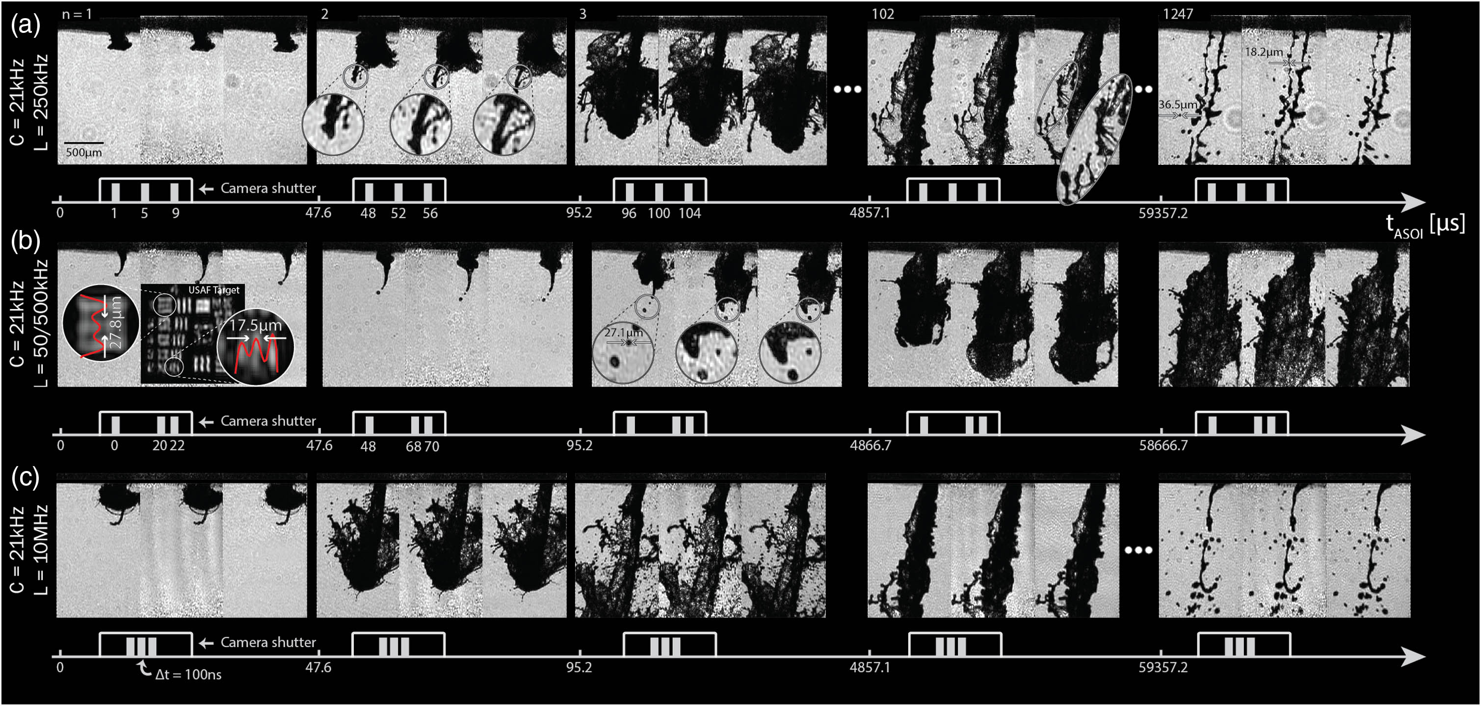
    Fig. 2. Microscopic imaging of transient fluid dynamics at high speed. (a) Imaging the spray injection event at a camera speed of 21 kHz and a shutter time of 12 μs within which three pulses, with constant inter-pulse time (250 kHz FRAME triplet), are recorded. (b) Non-linear temporal triggering where the first two pulses arrive at the sample with an inter-pulse time of 20 μs (50 kHz), while the last two are incident with an inter-pulse time of 2 μs (500 kHz). At the beginning of the event, 50 kHz suffices to track the fluid’s evolution within the camera exposure, while already at 95 μs ASOI, higher speeds are necessary. The zoom-ins of the USAF 1951 resolution target correspond to the resolution limits in x and y of the current optical configuration. (c) Imaging the injection event with 21 kHz camera speed and 10 MHz FRAME triplet (100 ns inter-pulse time) while retaining the image spatial resolution of (b). See Visualization 1, Visualization 2, Visualization 5, and Visualization 6 for videos of the entire events.
    Extracting 2D accelerometry data from a single camera exposure. (a) Thresholding and morphologically closing results in the green segmentation of the shadowgram. (b) Template matching between two frames results in 2D velocity vector fields (color coded arrows), calculated at the pixel level along the segmentation edge. Here we choose to calculate the vectors every fourth pixel, yielding a vector density of 0.25 px−1. Histogramming their sizes indicates downward movement towards the left (negative x direction but positive y direction) at an average speed of ∼102+152=18 m/s. (c) The matching of two velocity vector fields results in the acceleration (or, equivalently, force) fields that act upon the liquid body. The centering of the histograms around zero shows that the the vast majority of the spray does not accelerate. The Gaussian distribution of vectors, however, demonstrates the stochastic nature of the turbulence that is present. Furthermore, the zoom-in reveals a possible primary breakup event that is underway. (d) This process of force extraction is performed over the complete series of images from the start to the end of injection, showing the evolution of the spray’s dynamics for the entire event. The sensitivity of the system/algorithm is withheld for the varying velocity and acceleration regimes over the course of the event, from low to high velocity/acceleration at varying times. For a complete video of the injection event overlayed with accelerometry vectors, see Visualization 8.
    Fig. 3. Extracting 2D accelerometry data from a single camera exposure. (a) Thresholding and morphologically closing results in the green segmentation of the shadowgram. (b) Template matching between two frames results in 2D velocity vector fields (color coded arrows), calculated at the pixel level along the segmentation edge. Here we choose to calculate the vectors every fourth pixel, yielding a vector density of 0.25  px1. Histogramming their sizes indicates downward movement towards the left (negative x direction but positive y direction) at an average speed of 102+152=18  m/s. (c) The matching of two velocity vector fields results in the acceleration (or, equivalently, force) fields that act upon the liquid body. The centering of the histograms around zero shows that the the vast majority of the spray does not accelerate. The Gaussian distribution of vectors, however, demonstrates the stochastic nature of the turbulence that is present. Furthermore, the zoom-in reveals a possible primary breakup event that is underway. (d) This process of force extraction is performed over the complete series of images from the start to the end of injection, showing the evolution of the spray’s dynamics for the entire event. The sensitivity of the system/algorithm is withheld for the varying velocity and acceleration regimes over the course of the event, from low to high velocity/acceleration at varying times. For a complete video of the injection event overlayed with accelerometry vectors, see Visualization 8.
    Sensitivity of velocimetry to different inter-pulse durations. (a), (b) Two instances from one injection event are analyzed for three different, simultaneously acquired values of inter-pulse delay time (Δt). Intensity differences between the two individual images are depicted in blue and red, whereas black areas reflect static structures. The necessity of acquiring with multiple inter-pulse times is particularly clear for the yellow zoom-ins of (b). With a small Δt (i) the lack of structural change forces the velocity vectors to match with noise. However, as Δt increases (ii, iii), structural differences emerge, resulting in velocity vectors that are instead related to the spray dynamics. Similarly, the yellow zoom-ins of (a) show that the matching algorithm will give varying results for differing inter-frame times. In contrast, the two green zoom-ins depict structures with velocities that are more robust to such changes in Δt. The two instances together illustrate how the instabilities of the injected liquid may have different temporal characteristics throughout the duration of the event. These variations imply that a single, static value of Δt is not ideal to accurately track all the dynamics.
    Fig. 4. Sensitivity of velocimetry to different inter-pulse durations. (a), (b) Two instances from one injection event are analyzed for three different, simultaneously acquired values of inter-pulse delay time (Δt). Intensity differences between the two individual images are depicted in blue and red, whereas black areas reflect static structures. The necessity of acquiring with multiple inter-pulse times is particularly clear for the yellow zoom-ins of (b). With a small Δt (i) the lack of structural change forces the velocity vectors to match with noise. However, as Δt increases (ii, iii), structural differences emerge, resulting in velocity vectors that are instead related to the spray dynamics. Similarly, the yellow zoom-ins of (a) show that the matching algorithm will give varying results for differing inter-frame times. In contrast, the two green zoom-ins depict structures with velocities that are more robust to such changes in Δt. The two instances together illustrate how the instabilities of the injected liquid may have different temporal characteristics throughout the duration of the event. These variations imply that a single, static value of Δt is not ideal to accurately track all the dynamics.
    High-speed tracking of air resistance on a single droplet. (a) The direction of the forces acting on a single droplet, depicted by the solid yellow arrow (itself equal to the mean of the dashed arrows) indicates strong air resistance. (b) Despite this, the measured decrease in velocity from 46.7 to 24 m/s (depicted as a black circle) is less than expected from air resistance simulations performed using Stoke’s law and Schiller–Naumann (SN) correlation. Due to the deformation of the liquid droplet to a more aerodynamic shape (seen in the second velocity image), the correct drag coefficient is 15 times less than that proposed by SN correlation. See Appendix C for details.
    Fig. 5. High-speed tracking of air resistance on a single droplet. (a) The direction of the forces acting on a single droplet, depicted by the solid yellow arrow (itself equal to the mean of the dashed arrows) indicates strong air resistance. (b) Despite this, the measured decrease in velocity from 46.7 to 24 m/s (depicted as a black circle) is less than expected from air resistance simulations performed using Stoke’s law and Schiller–Naumann (SN) correlation. Due to the deformation of the liquid droplet to a more aerodynamic shape (seen in the second velocity image), the correct drag coefficient is 15 times less than that proposed by SN correlation. See Appendix C for details.
    19 MHz temporal resolution. (a) Due to their shape, the pulses from these nanosecond laser sources have a center of mass [red dashed line of inset] separated from the peak. Hence, the pulse limits (yellow dashed lines), within which 76% of the light intensity lies, are much further apart than the FWHM of the peak. Placing three such pulses in a pulse train, such that they adhere to the defined temporal resolution condition, allows for a 16 MHz pulse train. (b) Pulse limits versus FWHM: the asymmetric pulse shape of the lasers used here causes the pulse limits to be much larger than their Gaussian counterparts (red dots versus blue dots of the plot).
    Fig. 6. 19 MHz temporal resolution. (a) Due to their shape, the pulses from these nanosecond laser sources have a center of mass [red dashed line of inset] separated from the peak. Hence, the pulse limits (yellow dashed lines), within which 76% of the light intensity lies, are much further apart than the FWHM of the peak. Placing three such pulses in a pulse train, such that they adhere to the defined temporal resolution condition, allows for a 16 MHz pulse train. (b) Pulse limits versus FWHM: the asymmetric pulse shape of the lasers used here causes the pulse limits to be much larger than their Gaussian counterparts (red dots versus blue dots of the plot).
    Extraction of velocity vectors for each pixel along the segmentation edge. Two examples of where the initial template (green boxes) is scanned within a search area (red dashed boxes) across the subsequent image (outlined in orange). The template is placed at the position of maximum cross-correlation (orange boxes). The velocity vector is then calculated as the distance between the two center points divided by the inter-image time. This process is performed for every pixel along the segmentation edge.
    Fig. 7. Extraction of velocity vectors for each pixel along the segmentation edge. Two examples of where the initial template (green boxes) is scanned within a search area (red dashed boxes) across the subsequent image (outlined in orange). The template is placed at the position of maximum cross-correlation (orange boxes). The velocity vector is then calculated as the distance between the two center points divided by the inter-image time. This process is performed for every pixel along the segmentation edge.
    Validation of the velocity and acceleration extraction algorithm. (a) Experimental validation using the known gravitational acceleration acting upon a rigid sphere. The velocities are first extracted, yielding the displayed vector fields and distributions, where the angular distribution (θ) histogram is given by arctan(vx/vy) (a zero angle points directly in the direction of the fall). Matching the velocity vectors results in the extracted acceleration distribution with a mean acceleration of 9.74 m/s2 in the y direction and −0.2 m/s2 in the x direction. σax and σay correspond to a rounded two pixel uncertainty in the image segmentation process, while σθ corresponds to a single pixel uncertainty. (b) Synthetic data of a falling sphere (logical maps) accelerating at 9.82 m/s2 are inputted into the algorithm, resulting in distributions with zero width in velocities (magnitude and direction) and acceleration, validating the vector field extraction algorithm.
    Fig. 8. Validation of the velocity and acceleration extraction algorithm. (a) Experimental validation using the known gravitational acceleration acting upon a rigid sphere. The velocities are first extracted, yielding the displayed vector fields and distributions, where the angular distribution (θ) histogram is given by arctan(vx/vy) (a zero angle points directly in the direction of the fall). Matching the velocity vectors results in the extracted acceleration distribution with a mean acceleration of 9.74  m/s2 in the y direction and 0.2  m/s2 in the x direction. σax and σay correspond to a rounded two pixel uncertainty in the image segmentation process, while σθ corresponds to a single pixel uncertainty. (b) Synthetic data of a falling sphere (logical maps) accelerating at 9.82  m/s2 are inputted into the algorithm, resulting in distributions with zero width in velocities (magnitude and direction) and acceleration, validating the vector field extraction algorithm.
    Vassily Kornienko, David Andersson, Mehdi Stiti, Jonas Ravelid, Simon Ek, Andreas Ehn, Edouard Berrocal, Elias Kristensson. Simultaneous multiple time scale imaging for kHz–MHz high-speed accelerometry[J]. Photonics Research, 2022, 10(7): 1712
    Download Citation