• Photonics Research
  • Vol. 8, Issue 11, 1676 (2020)
Xiyuan Lu1、2、*, Ashutosh Rao1、3, Gregory Moille1、4, Daron A. Westly1, and Kartik Srinivasan1、4、5
Author Affiliations
  • 1Microsystems and Nanotechnology Division, Physical Measurement Laboratory, National Institute of Standards and Technology, Gaithersburg, Maryland 20899, USA
  • 2Institute for Research in Electronics and Applied Physics and Maryland NanoCenter, University of Maryland, College Park, Maryland 20742, USA
  • 3Department of Chemistry and Biochemistry, University of Maryland, College Park, Maryland 20742, USA
  • 4Joint Quantum Institute, NIST/University of Maryland, College Park, Maryland 20742, USA
  • 5e-mail: kartik.srinivasan@nist.gov
  • show less
    DOI: 10.1364/PRJ.401755 Cite this Article Set citation alerts
    Xiyuan Lu, Ashutosh Rao, Gregory Moille, Daron A. Westly, Kartik Srinivasan. Universal frequency engineering tool for microcavity nonlinear optics: multiple selective mode splitting of whispering-gallery resonances[J]. Photonics Research, 2020, 8(11): 1676 Copy Citation Text show less
    Illustration of MSMS. (a) Example of microring ring width modulation targeting m=6 and m=8 modes, with 20% and 10% of the nominal value (dashed line), respectively. This modulation selectively frequency-splits the (d) m=6 and (e) m=8 modes, while behaving as a normal microring with rotational symmetry for all other modes. We note that the m number and modulation amplitude are quite different than that implemented in real devices, for illustration purposes. (b) The modulation of the ring width for the MSMS device is plotted versus azimuthal angle in the top panel and has two frequency components in this case. The middle panel shows the modulation component targeting the m=6 mode with 20% modulation of the ring width, and the bottom panel shows the modulation component targeting the m=8 mode with 10% modulation of the ring width. (c) In the device transmission (top), this MSMS device introduces frequency splitting of the m=6 and m=8 modes, and the amplitude of the splittings linearly depends on their modulation amplitudes. This transmission trace is equivalent to the two individual SMS transmission traces (middle and bottom) together. (d) For the m=6 mode, the MSMS device is equivalent to the SMS device described by the (6, 0.2) modulated boundary (blue). Degenerate CW and CCW modes are renormalized to two standing-wave modes. The standing-wave mode that always experiences a wider ring width has a larger resonance wavelength, and therefore a redshifted resonance frequency. The other mode always experiences a narrower ring width and is blueshifted. (e) For the m=8 mode, the MSMS device behaves as the SMS device described by the (8, 0.1) boundary (red). (f) For other modes (m≠{6,8}), for example, m=9, the MSMS device does not induce coherent scattering, and therefore behaves similarly to a rotationally symmetric ring (dashed line).
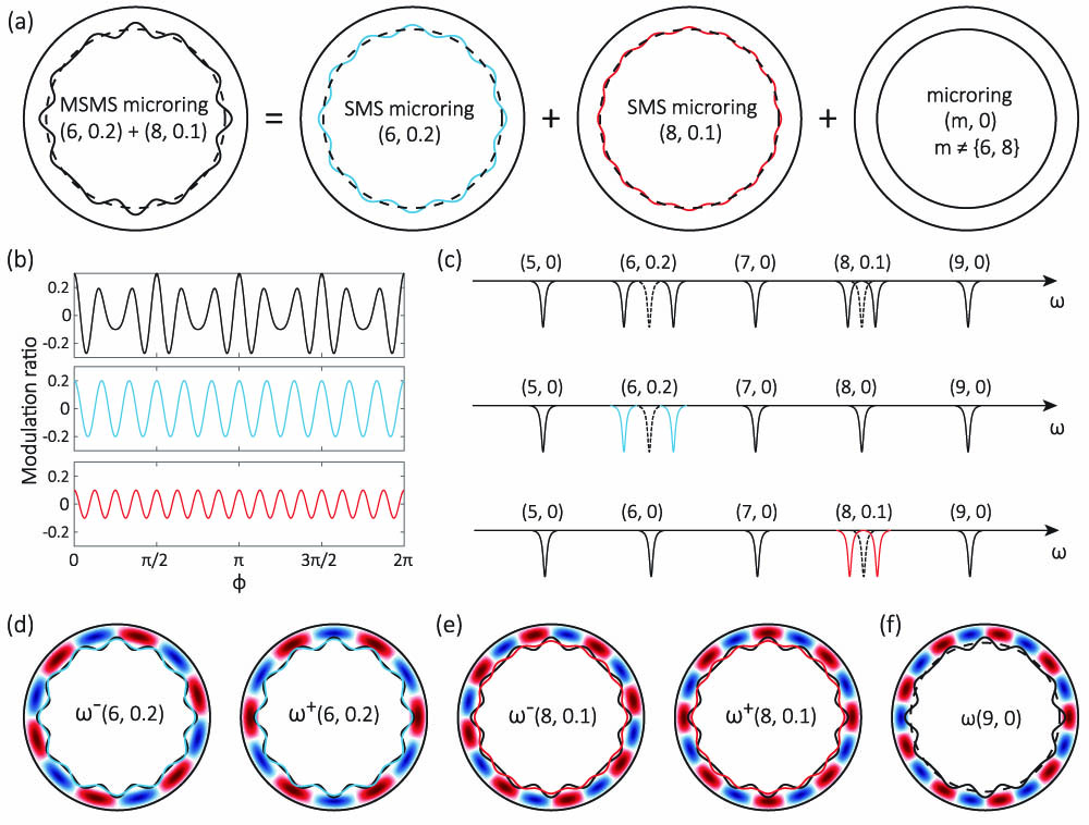
    Fig. 1. Illustration of MSMS. (a) Example of microring ring width modulation targeting m=6 and m=8 modes, with 20% and 10% of the nominal value (dashed line), respectively. This modulation selectively frequency-splits the (d) m=6 and (e) m=8 modes, while behaving as a normal microring with rotational symmetry for all other modes. We note that the m number and modulation amplitude are quite different than that implemented in real devices, for illustration purposes. (b) The modulation of the ring width for the MSMS device is plotted versus azimuthal angle in the top panel and has two frequency components in this case. The middle panel shows the modulation component targeting the m=6 mode with 20% modulation of the ring width, and the bottom panel shows the modulation component targeting the m=8 mode with 10% modulation of the ring width. (c) In the device transmission (top), this MSMS device introduces frequency splitting of the m=6 and m=8 modes, and the amplitude of the splittings linearly depends on their modulation amplitudes. This transmission trace is equivalent to the two individual SMS transmission traces (middle and bottom) together. (d) For the m=6 mode, the MSMS device is equivalent to the SMS device described by the (6, 0.2) modulated boundary (blue). Degenerate CW and CCW modes are renormalized to two standing-wave modes. The standing-wave mode that always experiences a wider ring width has a larger resonance wavelength, and therefore a redshifted resonance frequency. The other mode always experiences a narrower ring width and is blueshifted. (e) For the m=8 mode, the MSMS device behaves as the SMS device described by the (8, 0.1) boundary (red). (f) For other modes (m{6,8}), for example, m=9, the MSMS device does not induce coherent scattering, and therefore behaves similarly to a rotationally symmetric ring (dashed line).
    1SMS. (a) Transmission scans for four devices with different modulation amplitudes, where the labels (m, A) represent the azimuthal mode number m and the (nominal) modulation amplitude A in nanometers. In the top panel, the control device without SMS shows a cavity transmission spectrum without frequency splitting for any of the modes. From the second panel down, the devices exhibit a transmission spectrum with increasing frequency-splitting for the targeted m=163 mode, with a splitting proportional to the prescribed modulation amplitude. Besides the TE1 modes under investigation, another set of modes appears, which is verified to be fundamental transverse-magnetic modes (TM1). The appearance of these modes is due to wavelength-dependent polarization rotation in the fibers used, which could be resolved by using polarization-maintaining fibers. (b) The top panel shows that the amount of mode splitting is linearly proportional to the modulation amplitude and reaches a value of ≈0.8 nm. The bottom panel shows that the adjacent four modes have much smaller splitting (<7.5% of the targeted mode, that is, below the black line) than the targeted modes. In both panels the uncertainties in the mode splitting, determined from nonlinear least squares fits to the data, are smaller than the data point size. (c) Transmission spectrum and fit trace of the singlet resonance without mode splitting, (163, 0), where Q0 is the intrinsic optical quality factor. (d) Transmission spectrum for the doublet resonance (163, 3), with an observable mode splitting that is a couple of times the mode linewidths. From these linewidths, we determine Q0+ and Q0−, the intrinsic optical quality factors for the blueshifted and redshifted modes, respectively. The differences in the coupling and intrinsic Qs for these two modes are potentially due to the different localization of the two standing-wave modes with respect to the ring-waveguide coupling region and possible point defects, respectively. (e) and (f) Two doublet resonances (163, 9) and (163, 21) that are well separated (262 pm and 591 pm splitting, respectively). See Appendix C for fitting methods.
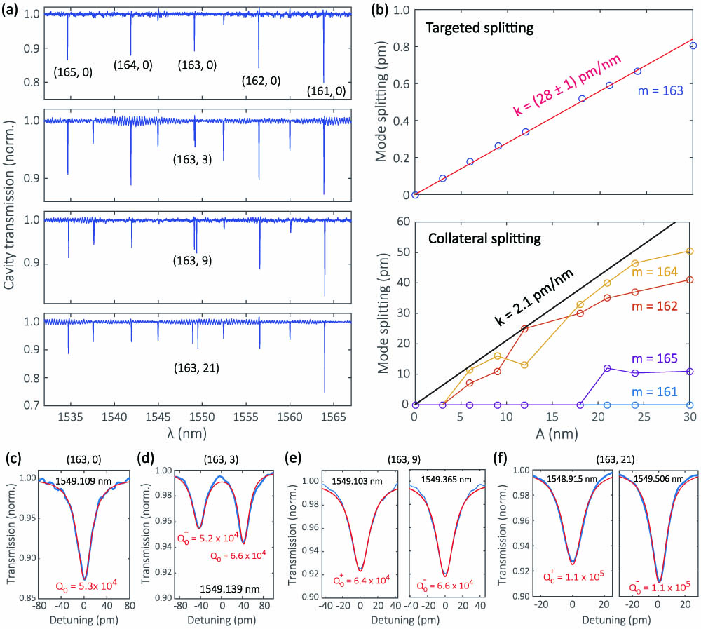
    Fig. 2. 1SMS. (a) Transmission scans for four devices with different modulation amplitudes, where the labels (m, A) represent the azimuthal mode number m and the (nominal) modulation amplitude A in nanometers. In the top panel, the control device without SMS shows a cavity transmission spectrum without frequency splitting for any of the modes. From the second panel down, the devices exhibit a transmission spectrum with increasing frequency-splitting for the targeted m=163 mode, with a splitting proportional to the prescribed modulation amplitude. Besides the TE1 modes under investigation, another set of modes appears, which is verified to be fundamental transverse-magnetic modes (TM1). The appearance of these modes is due to wavelength-dependent polarization rotation in the fibers used, which could be resolved by using polarization-maintaining fibers. (b) The top panel shows that the amount of mode splitting is linearly proportional to the modulation amplitude and reaches a value of 0.8  nm. The bottom panel shows that the adjacent four modes have much smaller splitting (<7.5% of the targeted mode, that is, below the black line) than the targeted modes. In both panels the uncertainties in the mode splitting, determined from nonlinear least squares fits to the data, are smaller than the data point size. (c) Transmission spectrum and fit trace of the singlet resonance without mode splitting, (163, 0), where Q0 is the intrinsic optical quality factor. (d) Transmission spectrum for the doublet resonance (163, 3), with an observable mode splitting that is a couple of times the mode linewidths. From these linewidths, we determine Q0+ and Q0, the intrinsic optical quality factors for the blueshifted and redshifted modes, respectively. The differences in the coupling and intrinsic Qs for these two modes are potentially due to the different localization of the two standing-wave modes with respect to the ring-waveguide coupling region and possible point defects, respectively. (e) and (f) Two doublet resonances (163, 9) and (163, 21) that are well separated (262 pm and 591 pm splitting, respectively). See Appendix C for fitting methods.
    5SMS. (a) Cavity transmission traces of five devices with different configurations of 5SMS. Each split mode is labeled by (m, A), with A in units of nanometers. (b) The measured mode-splitting amounts clearly correspond to the expected modulation pattern, where A=15 nm and A=5 nm ring width modulation amplitudes correspond to (390±20) pm and (140±10) pm mode splittings, while the untargeted modes have ≈7% collateral splitting. The slopes (splitting divided by the modulation amplitude) are (26±1) pm/nm and (28±2) pm/nm, respectively, close to the 1SMS slope in Fig. 2(b). The uncertainties in mode splitting are smaller than the data point size. (c) Typical example of the cavity transmission for a targeted mode with 408 pm mode splitting; (d) typical example of the cavity transmission of a targeted mode with 140 pm mode splitting; (e) the average of the intrinsic optical quality factors of all the modes in these 5SMS devices is, surprisingly, more than 1 standard deviation higher than the average in the 1SMS devices (red open circles). Qs for individual modes are shown as solid blue dots. We note that the Qs of 1SMS modes are generally higher with >20 nm modulation amplitude (see Appendix A). The 3SMS devices (where three modes are targeted for mode splitting) have Qs that are in-between the 1SMS and 5SMS cases (see Appendix B).
    Fig. 3. 5SMS. (a) Cavity transmission traces of five devices with different configurations of 5SMS. Each split mode is labeled by (m, A), with A in units of nanometers. (b) The measured mode-splitting amounts clearly correspond to the expected modulation pattern, where A=15  nm and A=5  nm ring width modulation amplitudes correspond to (390±20)  pm and (140±10)  pm mode splittings, while the untargeted modes have 7% collateral splitting. The slopes (splitting divided by the modulation amplitude) are (26±1)  pm/nm and (28±2)  pm/nm, respectively, close to the 1SMS slope in Fig. 2(b). The uncertainties in mode splitting are smaller than the data point size. (c) Typical example of the cavity transmission for a targeted mode with 408 pm mode splitting; (d) typical example of the cavity transmission of a targeted mode with 140 pm mode splitting; (e) the average of the intrinsic optical quality factors of all the modes in these 5SMS devices is, surprisingly, more than 1 standard deviation higher than the average in the 1SMS devices (red open circles). Qs for individual modes are shown as solid blue dots. We note that the Qs of 1SMS modes are generally higher with >20  nm modulation amplitude (see Appendix A). The 3SMS devices (where three modes are targeted for mode splitting) have Qs that are in-between the 1SMS and 5SMS cases (see Appendix B).
    Microring-waveguide coupling. (a) In an MSMS device, targeted modes become standing waves that equally comprise a CCW (red) part and a CW (black) part. Assuming a undirectional waveguide input as shown in the diagram, the CCW part can be coupled to at a rate Γc=Γccw, while the CW part is not directly coupled to the waveguide because of the large momentum mismatch from the input light (Γc=0). The MSMS modes are therefore expected to have an overall coupling rate of Γc=Γccw/2 in theory. (b) Considering a 5SMS device in which the m={159,161,163,165,167} modes are targeted, the measured Qc (blue) is clearly larger for the split modes (each indicated by a black dashed line) than for other modes, and therefore Qc as a function of azimuthal mode order shows an oscillatory behavior. Dividing Qc for the split modes by 2 yields inferred values of their CCW coupling Q (red), which are similar to those of the unsplit modes. This trend is consistent with the prediction in (a), as Qc=ω/Γc. Error bars are 1 standard deviation values resulting from nonlinear least squares fits to the data.
    Fig. 4. Microring-waveguide coupling. (a) In an MSMS device, targeted modes become standing waves that equally comprise a CCW (red) part and a CW (black) part. Assuming a undirectional waveguide input as shown in the diagram, the CCW part can be coupled to at a rate Γc=Γccw, while the CW part is not directly coupled to the waveguide because of the large momentum mismatch from the input light (Γc=0). The MSMS modes are therefore expected to have an overall coupling rate of Γc=Γccw/2 in theory. (b) Considering a 5SMS device in which the m={159,161,163,165,167} modes are targeted, the measured Qc (blue) is clearly larger for the split modes (each indicated by a black dashed line) than for other modes, and therefore Qc as a function of azimuthal mode order shows an oscillatory behavior. Dividing Qc for the split modes by 2 yields inferred values of their CCW coupling Q (red), which are similar to those of the unsplit modes. This trend is consistent with the prediction in (a), as Qc=ω/Γc. Error bars are 1 standard deviation values resulting from nonlinear least squares fits to the data.
    Nonlinear optics applications for the two-mode selective mode splitting (2SMS) case. (a) In the case of a conventional WGM microcavity (left column), realizing an efficient parametric nonlinear process relies on finding a device geometry whose global dispersion profile results in frequency matching for the modes of interest for a given nonlinear optical process, e.g., (I) intraband and (II) interband frequency conversion via FWM-BS, and (III) photon-pair generation. (b) In contrast, by using a 2SMS device (right column), frequency matching can be achieved without any specific consideration of the global dispersion profile (and hence the resonator cross section), so that any of the displayed nonlinear processes can be achieved. For intraband FWM-BS in a conventional microcavity [I(a)], global dispersion engineering typically leads to an unwanted conversion channel (dashed arrow) along with the targeted channel (solid arrow). But in an MSMS cavity, FWM-BS naturally occurs for only a single set of modes [solid arrows in I(b)]. Moreover, MSMS modes can be used in flexible ways, either exclusively MSMS modes [I(b)1], or combined with unsplit modes [I(b)2]. This MSMS cavity can also be applied to interband FWM-BS (II) and nondegenerately pumped photon pair generation (III) in similar ways, not only relaxing the frequency engineering for the targeted process (solid arrows), but also enabling suppression of the unwanted process [dashed arrows in I(a)–III(a)].
    Fig. 5. Nonlinear optics applications for the two-mode selective mode splitting (2SMS) case. (a) In the case of a conventional WGM microcavity (left column), realizing an efficient parametric nonlinear process relies on finding a device geometry whose global dispersion profile results in frequency matching for the modes of interest for a given nonlinear optical process, e.g., (I) intraband and (II) interband frequency conversion via FWM-BS, and (III) photon-pair generation. (b) In contrast, by using a 2SMS device (right column), frequency matching can be achieved without any specific consideration of the global dispersion profile (and hence the resonator cross section), so that any of the displayed nonlinear processes can be achieved. For intraband FWM-BS in a conventional microcavity [I(a)], global dispersion engineering typically leads to an unwanted conversion channel (dashed arrow) along with the targeted channel (solid arrow). But in an MSMS cavity, FWM-BS naturally occurs for only a single set of modes [solid arrows in I(b)]. Moreover, MSMS modes can be used in flexible ways, either exclusively MSMS modes [I(b)1], or combined with unsplit modes [I(b)2]. This MSMS cavity can also be applied to interband FWM-BS (II) and nondegenerately pumped photon pair generation (III) in similar ways, not only relaxing the frequency engineering for the targeted process (solid arrows), but also enabling suppression of the unwanted process [dashed arrows in I(a)–III(a)].
    1SMS Q analysis. (a) The intrinsic optical Qs of the SMS modes (red and blue) are consistent with the values from untargeted modes (gray data indicate 1 standard-deviation range given by fits to the four adjacent resonances). (b) The coupling Qs of the SMS modes (red and blue) are statistically larger than the values from untargeted modes (1 standard-deviation range found by fits of the four adjacent resonances shown in gray), as expected based on their standing-wave nature. Dividing the coupling Q of the targeted modes by two gives values (indicated by the red and blue dashed lines) that are within the range of Q values from other modes, consistent with expectation from theory.
    Fig. 6. 1SMS Q analysis. (a) The intrinsic optical Qs of the SMS modes (red and blue) are consistent with the values from untargeted modes (gray data indicate 1 standard-deviation range given by fits to the four adjacent resonances). (b) The coupling Qs of the SMS modes (red and blue) are statistically larger than the values from untargeted modes (1 standard-deviation range found by fits of the four adjacent resonances shown in gray), as expected based on their standing-wave nature. Dividing the coupling Q of the targeted modes by two gives values (indicated by the red and blue dashed lines) that are within the range of Q values from other modes, consistent with expectation from theory.
    3SMS results. (a) Cavity transmission for four devices with different configuration of 3SMS. The modulated modes are labeled as (m, A), where m represents the azimuthal mode number, and A represents its modulation amplitude in nanometers. (b) The measured mode splittings clearly show the targeted control of three modes with a splitting amplitude proportional to the modulation amplitude. (c)–(e) Optical Q fitting examples for modulation amplitudes of 15 nm, 5 nm, and 0 nm, respectively.
    Fig. 7. 3SMS results. (a) Cavity transmission for four devices with different configuration of 3SMS. The modulated modes are labeled as (m, A), where m represents the azimuthal mode number, and A represents its modulation amplitude in nanometers. (b) The measured mode splittings clearly show the targeted control of three modes with a splitting amplitude proportional to the modulation amplitude. (c)–(e) Optical Q fitting examples for modulation amplitudes of 15 nm, 5 nm, and 0 nm, respectively.
    High-Q 1SMS devices. (a) An optimized etching process leads to a device with intrinsic Q of 2.5×10⁵ for a mode with a 1.75 nm splitting. (b) With postprocessing steps consisting of annealing and dilute hydrofluoric acid etching, the device has shifted resonances with intrinsic Q improved to 7.6×10⁵ and decreased splitting of 1.62 nm.
    Fig. 8. High-Q 1SMS devices. (a) An optimized etching process leads to a device with intrinsic Q of 2.5×10⁵ for a mode with a 1.75 nm splitting. (b) With postprocessing steps consisting of annealing and dilute hydrofluoric acid etching, the device has shifted resonances with intrinsic Q improved to 7.6×10⁵ and decreased splitting of 1.62 nm.
    Xiyuan Lu, Ashutosh Rao, Gregory Moille, Daron A. Westly, Kartik Srinivasan. Universal frequency engineering tool for microcavity nonlinear optics: multiple selective mode splitting of whispering-gallery resonances[J]. Photonics Research, 2020, 8(11): 1676
    Download Citation