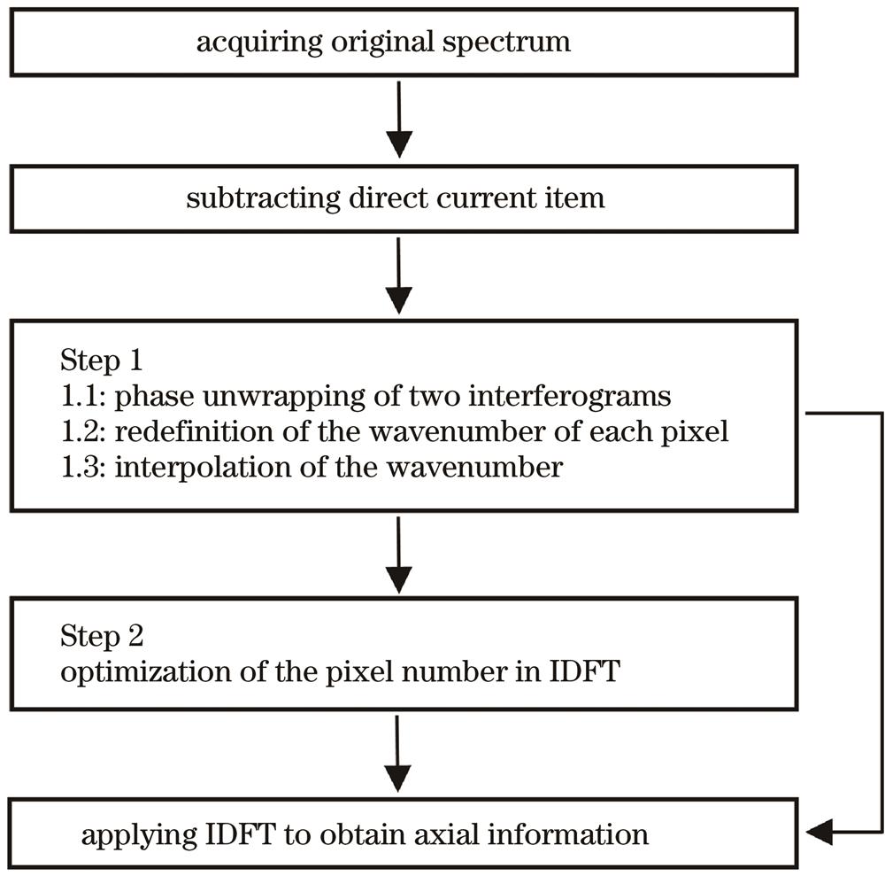
Fig. 1. Numerical processing flow of the whole algorithm

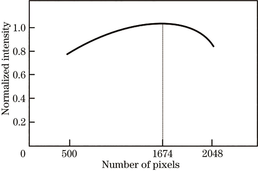
Fig. 2. Normalized intensity varing with pixel number when performing IDFT to the fringe pattern

Fig. 3. Detail of axial profiles of three optimization methods. (a) Comparison of ten axial reflectance profiles in a logarithmic scale when a reflector performs as the sample; (b) enlarged inset that is from the box of Fig. 3 (a)

Fig. 4. The cross-sectional images of Scotch tape. (a) The IDFT is performed when the interpolation is applied based on two interferograms; (b) the IDFT is performed following after the optimization of pixel number; (c) the result is performed based on the empirical optimization method; (d) the signal intensity of five different positions marked in Fig. 4 (a)-(c), EO is empirical optimization

Fig. 5. Percentage of pixel number from Fig. 4(a)-(c) that the pixel intensity ranges in top 20%, top 20%-40%, and residual 60%

Fig. 6. The cross-sectional images of multilayer glass slices. (a) The IDFT is performed when the interpolation is applied based on two interferograms; (b) the IDFT is performed after the optimization of pixel number; (c) the result is realized based on the empirical optimization method; (d) the signal sensitivity of five different positions marked in Fig. 6(a)-(c)

Fig. 7. Percentage of pixel number from Fig. 6(a)-(c) that the pixel intensity ranges in top 20%, top 20%-40%,and residual 60%