Fourier domain optical coherence tomography（FDOCT）enables three-dimensional（3D）imaging while light penetrates near-surface of a sample and it exploits an interferometric detection of broadband backscattered light. The axial profiles make FDOCT superior to the conventional microscope as well as FDOCT has better lateral resolution due to the confocal gate，which is critical to detect the micron-level defects and diagnose the early lesions in the body^［1-3］. The components of FDOCT usually incorporate a broadband light source，a Michelson interferometer，and a spectrometer. The spectra of light originating from two arms are interfered and captured. The interference patterns have three terms，including background of reference beam，autocorrelation of sample，and the cross term，where the last portion is encoded with the axial reflectance we desire. The cross term of the interference fringes is expressed as A（Δz）·cos（2k·Δz），where A（Δz）is the reflectance at the depth of Δz with respect to the reference mirror and k is the wavenumber. The wavenumber function and the depth function compose a Fourier transform pair^［4］. Employed with a broadband light，the axial reflectance profile can be obtained through performing inverse discrete Fourier transform（IDFT）to the spectra that are captured in a spectrometer. In fact，the difference of optical properties or optical thicknesses of the elements in two arms results in the dispersion dismatch where the fringes could be observed as Δz equals to zero. Such phenomenon makes the cross term add a new phase component that is related to the wavenumber，which blurs the axial point spread function of the reflector. The quantification of dispersion delay was represented by the Taylor expansion and the coefficients were determined by using the iteration algorithm to sharpen the vertical image^［4-5］. Also，Fercher et al. proposed the convolution with depth variant kernel to compensate dispersion^［6］. In addition，the utilization of the same components in two light paths eliminated the dispersion delay^［7-9］. In a grating-based spectrometer，the spectrum is sampled in wavelength domain that is evenly resampled in k domain，and the spectral calibration method based on the characteristic spectra of a heated light was employed^［10］，which makes the calibration procedure be complicated and redundant. What’‍s more，with the knowledge of the pixel coordinates of one or two wavelengths and the interferograms at two depths，the high-precision performance of wavelength calibration was realized^［11-12］. However，the priori condition of the pixel orientation of at least one wavelength is inevitable. As we know，the mechanical offset error of setup is ineradicable，which has impact on the accuracy of the spectrometer. Reducing the procedures above while increasing the image quality would help the buildup of FDOCT system more practical，the aim of which is an urgent demand.

In the paper，we propose and demonstrate a numerical post-processing flow from original spectral interferograms to the B-scan images in FDOCT system. First，the uniform sampling of the cross term in k domain is performed using two interferograms where the spectrum calibration is canceled，and the spectral dispersion delay has no impact on the method. Then，the sampling number in IDFT is optimized to maximize the sensitivity in the cross-sectional images. Compared with the empirical optimization method^［13］，the sensitivity of the proposed method is improved by 1.62 dB. The advantage of the method here has no knowledge of the pixel coordinates of any wavelength in the spectrometer while the spectra displacement results in the decrease of the sensitivity based on conventional technique^［14］. The cross-sectional images of Scotch tape and multilayer glass slices are tested and the sharper and more details are observed.

A homemade FDOCT apparatus is used here^［15］. In our FDOCT system，consisting of a broadband light source and a Michelson interferometer，the desired term on the camera is expressed as follows：

Where，A（Δz）is the axial reflectance at the depth of Δz with respect to the reference mirror； I（k）is the intensity of the fringes that is normalized from the spectral density distribution of the light source； x_i is the ith pixel（i = 1，2，…，N）； N is the pixel number for recording the spectra； φ_d（k）is the dispersion delay of two arms in the interferometer； φ_n is the phase noise. In the reference arm，we axially translate the optical elements（including objective and mirror that are mounted on a manual stage with a micrometer）to two positions with the movement of Δz´，and two interferograms are captured. In the spectrometer，the pixel coordinates of wavelengths are independent of the layout of optical elements in the interferometer. To unwrap the phase of two interference fringes，the Hilbert transform is performed on the interferograms，and the phase distribution of the fringes satisfies with the following expression：

Where，I˜[k(xi)] is the Hilbert transform of I[k(xi)]. The phase difference occurring in two interferograms abides by

The movement of Δz´ is read from the micrometer of the one-axis stage. It should be noted that the dispersion delay remains at two axial positions and it is removed in the Eq.（3）. Ignoring the phase noise，the wavenumber as the function of pixel coordinates obeys with the equation as follows：

Different from the reported method^［13］，we randomly assign one wavelength（e.g.，λ= 550 nm）at pixel x_j（j∈｛1，2，…，2048｝，e.g.，j=1000），and then the pixel coordinates of whole wavelengths are available based on the Eq.（4）. In point of physics，the coordinates of actual wavelength are not consistent with that we assign. However，the IDFT of the interference fringes has no relation to the actual wavelengths，which only needs to be evenly sampled in k domain based on the Fourier analysis of signal. Here the lack of physical spectra calibration helps improve the accuracy of the k-domain sampling of the interferograms. Also，the acquisition of coordinates of all wavelengths has no concern with the dispersion delay based on the Eq.（3）. We could observe that the spacing in k domain in the Eq.（4） is nonuniform. Following the Eq.（1），the interpolation of the spectral fringes should be applied to ensure the fringes pattern distributes as the function of the uniformly spaced wavenumbers before performing IDFT. The cubic spline interpolation is used to the original spectral intensity I（k）based on a set of k´（x_i）that has the identical spacing determined by（k_max-k_min）/N. Then a new interference term is achieved：

It is well known that the dispersion delay has impact on the axial sharpness. And we choose the hardware method to balance dispersion mismatch where two arms have the same optical elements，including neutral density filters and objectives. As a result，the component φ_d（k´）is eliminated from the Eq.（5） and the interference term is expressed as follows：

As far as we know，the axial reflectance profile in FDOCT is achieved through executing an IDFT to the interference spectra. The expression of IDFT to the cross term is

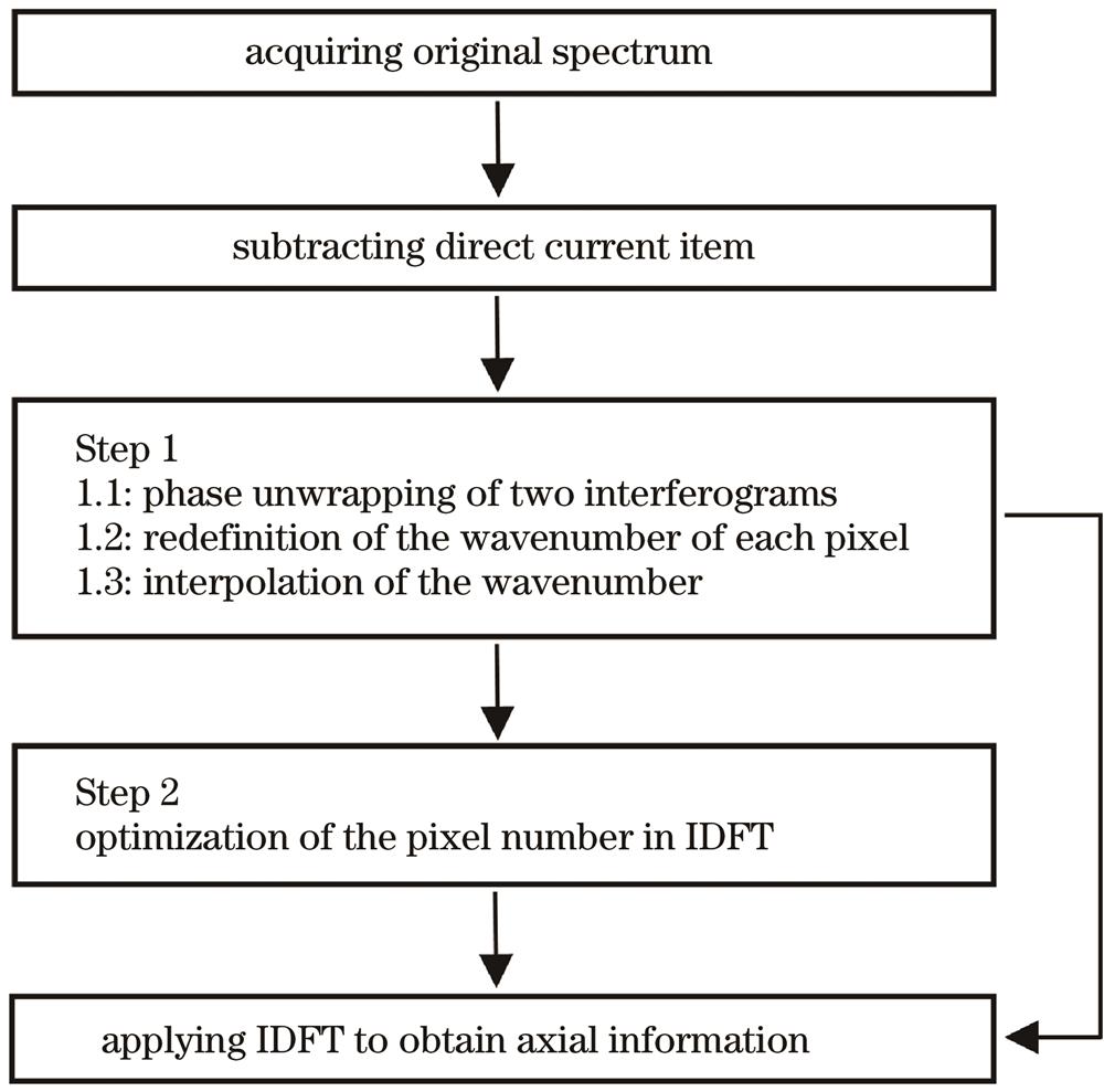
where i（Δz）is the reflectance at the depth of Δz. From the Eq.（7），the fact is that the outcome of IDFT is sensitive to the pixel number N. With different pixel number，the errors in the summation based on computer make an impact on the frequencies of fringes. In addition，the phase error decreases while the pixel number is reduced. In the process of IDFT to the interference fringes，the pixel number is optimized to maximize the sensitivity here. The whole algorithm process above is shown in Fig. 1.

Beginning from the original spectrogram，all the steps are accomplished through numerical calculation，where no hardware elements（i.e.，optical filters）are employed to calibrate the optical system. To explore the feasibility of the proposed method，the specula serve as the sample. In our experiment，the axial offsetΔz´ is 50 μm and we assign the wavenumber of 2.02 μm^-1 to the pixel 1000th. During the whole 2048 pixels，the maximal wavenumber and the minimal wavenumber are 3.92 μm^-1 and 0.01 μm^-1 respectively. Based on the algorithm of Step 1，we calculate that the physical sampling interval of each pixel is 1.61 μm，which is superior to the empirical optimization method that has no understanding of the actual depth^［13］. The pixel number used for the IDFT starts from the original 2048 pixels and the drop step is 20. Also，the window of the cropped spectrum is moved from the first pixel to the end. The normalized sensitivity with respect to the pixel number is shown in Fig. 2. Using the first 1674 pixels，the peak intensity is 1.45 times higher than that using the whole 2048 pixels. As shown in Fig. 3（a），ten axial positions using a reflector are reconstructed，where the depth interval is 50 μm. The black lines display ten axial reflectance profiles that the spectrogram is uniformly discretized in k-domain followed by IDFT. The blue lines display ten axial reflectance profiles that is achieved by the empirical optimization method，which almost overlap with the black lines. The red lines display ten axial reflectance profiles where the optimization of pixel number is implemented. The sensitivity of reflectance profiles is presented in logarithm. Fig. 3（b）is enlarged from the dashed box of Fig. 3（a），the peak of red line is 1.62 dB higher than that of black line.

To demonstrate the ability of the numerical reconstruction of vertical image，Scotch tape is used to display the changes in the cross-sectional images，which is shown in Fig. 4. In Fig. 4（a），the vertical image of the Scotch tape is reconstructed from the interpolation of spectrogram based on Step 1. Taking advantage of our two-step procedure，Fig. 4（b）shows the vertical image with the combination of Step 1 and Step 2. Fig. 4（c）exhibits the vertical image via the empirical optimization method. As we know，the high intensity represents the reflectance that is encoded with the structure of layers，and such signal is what we desire. The signal sensitivity of five specific positions marked in Fig. 4（a）-（c）is compared and the result shown in Fig. 4（d）demonstrates the optimization of Step 2 improves the signal sensitivity. To well explain the quality of images overall，we count the pixel number at three levels of intensity that is shown in Fig. 5. First，we normalize the intensity of three images in Fig. 4（a）-（c）. We compute the percentage of pixel number in three images when the intensity ranges in top 20%，top 20%-40%，and residual 60%，respectively. The percentage of pixel number where the pixel intensity belongs to the top 20% in Fig. 4（b），Fig. 4（a），and Fig. 4（c）is 5.21%，4.20%，and 2.70%. The percentage of pixel number that the pixel intensity situates in the top 20%-40% in Fig. 4（b），Fig. 4（a），and Fig. 4（c）is 60.07%，57.09%，and 31.31%. The pixel intensity ranging in the residual 60% is not high enough to show the details of the vertical images.

A stack of glass slices is also used to verify the performance of our methods，which is shown in Fig. 6. Seven slices are imaged and six lines are observed. Fig. 6（a）is achieved based on the interpolation of fringes（Step 1）. And Fig. 6（b）displays the cross-sectional image via the optimization of Step 2. Fig. 6（c）shows the reconstructed image based on the empirical optimization method. As shown in Fig. 6（d），the signal sensitivity of five specific positions marked in Fig. 6（a）-（c）is also compared and the result demonstrates the optimization of Step 2 improves the signal sensitivity. We also count the percentage of pixel number at three levels of intensity in Fig. 6（a）-（c）. As shown in Fig. 7，the percentage of pixel number that the pixel intensity distributes in the top 20% in Fig. 6（b），Fig. 6（a），and Fig. 6（c）is 7.73%，6.16%，and 1.46%. The percentage of pixel number that the pixel intensity situates in the top 20%-40% in Fig. 6（b），Fig. 6（a），and Fig. 6（c）is 62.32%，56.91%，and 36.54%. Here we also see that the pixel percentage of high intensity in Fig. 6（b）-（c）ranks in the descending order.

A data post processing flow is demonstrated to reconstruct the cross-sectional images in FDOCT system. Different from the conventional methods of spectrum calibration，the uniform discretization in k domain is performed using two interferograms. Such a way depends on the numerical analysis without calibrating any wavelength and the precision of the pixel distribution of wavenumber is higher than that of the conventional spectrometer due to the mechanical shift of the optical elements，e.g.，the grating. Besides，the optimization of pixel number helps improve the quality of cross-sectional images，that is critical to the inspection of all kinds of purposes，including impurities，defect，diseases and so on.