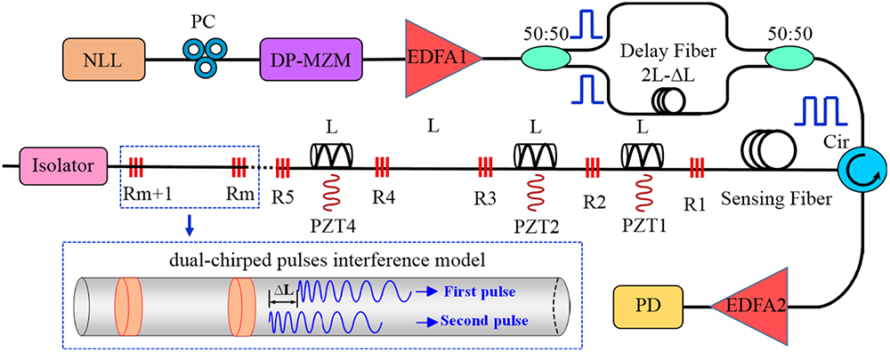
Fig. 1. Schematic diagram of a WFBGs array system.

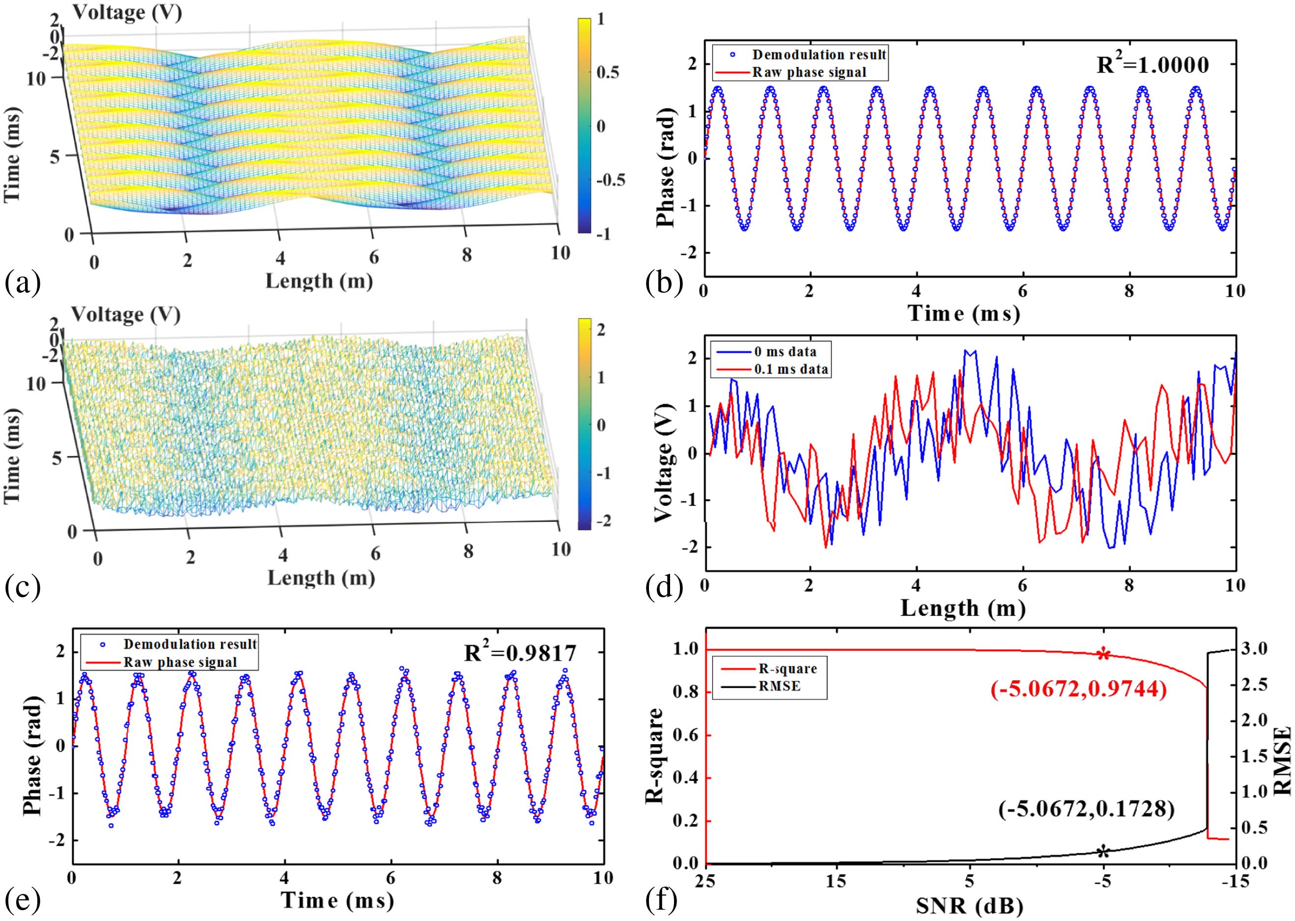
Fig. 2. DFT simulation results. (a) 3D spatial-temporal profile of original a 20 MHz sinusoidal signal with a varying phase without noise. (b) Phase demodulation result of a 20 MHz sinusoidal signal without noise. (c) 3D spatial-temporal profile of a 20 MHz noise-added sinusoidal signal with a varying phase. (d) Two noise-added signal traces at the moments of t=0 and t=0.1  ms. (e) Phase demodulation result of a 20 MHz noise-loaded sinusoidal signal. (f) R-squared and RMSE of phase demodulation results at different SNRs.

Fig. 3. Raw beat frequency signal at 2 km. (a) 3D spatial-temporal profile at the sensing section. (b) All-fiber signal at the moment t=0 and t=0.1  ms. (c) Sensing section signal at the moment t=0 and t=0.1  ms.

Fig. 4. Phase demodulation results of different types of PZTs. (a) Reconstructed signal waveforms for PZT1 at different voltages. (b) Demodulation results and fitting curves of different amplitude signals for PZT1. (c) Reconstructed signal waveforms for PZT2 at different voltages. (d) Demodulation results and fitting curves of different amplitude signals for PZT2.

Fig. 5. Time-domain and frequency-domain plots of PZT at different frequencies. (a) Time-domain information of the phase demodulation result of the 0.8 kHz signal. (b) Time-domain information of phase demodulation result of the 1.0 kHz signal. (c) Time-domain information of phase demodulation result of the 1.2 kHz signal. (d) Frequency-domain information of demodulation results for 0.8, 1.0, and 1.2 kHz signals.

Fig. 6. Raw beat frequency signal and phase demodulation results at 101 km. (a) 3D spatial-temporal profile at the sensing section. (b) Sensing section signal and power spectrum at the moment t=0 and t=0.1  ms. (c) The signal demodulation result of the sensing section 1. (d) The signal demodulation result of the sensing section 2.