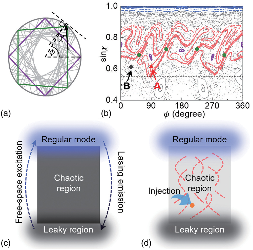
Fig. 1. (a) Chaotic ray dynamics in an asymmetric microcavity in real space. Green lines and purple lines are unstable four-period orbit and stable four-period orbit, respectively. ϕ: azimuthal angle. χ: incident angle. (b) The phase space of the chaotic microcavity. Blue points: KAM curves. Green dots: four-period unstable orbit. Purple dots: four-period stable orbit. Red points: stable manifold. Black dashed line: critical line. Point A: (90°, 0.61), near the stable manifold in the chaotic region. Point B: (30°, 0.61), in the chaotic region away from the stable manifold. (c) Investigation of the chaotic dynamics by lasing emission or free-space coupling between regular mode and leaky region, where the chaotic region is treated as a “black box.” (d) Probing the stable manifold by precisely controlling the injection position in phase space.

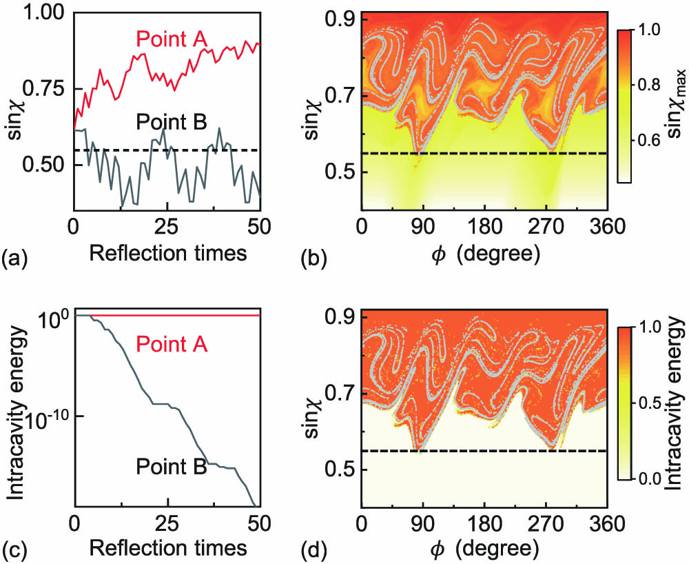
Fig. 2. (a) Angular momentum sin χ versus reflection times starting from point A and point B as shown in Fig. 1(b). (b) Maximal angular momentum sin χmax distribution within 50 reflections by the ray model. Gray dots: stable manifold of the four-period unstable orbit. (c) Energy intensity versus reflection times starting from point A and point B. (d) Intracavity energy distribution within 50 reflections by the ray model.

Fig. 3. (a) Schematic illustration of the fiber–cavity coupling setup. Inset: scanning electron microscope image of the fiber with a diameter of D. (b) Typical experimental transmission spectra at different azimuthal angles (ϕ=30°, 60°, 90°) with nanofiber diameter of 415 nm. The right panel is the zoom-in blue shadow in the spectra. The dashed line marks a same high-Q mode. The coupling depth is denoted by h.

Fig. 4. (a), (b) Experimental output power (gray histograms) versus the excitation azimuthal angles in experiments with nanofiber diameters of 415 nm and 530 nm, respectively. The waterfall plots present corresponding intracavity energy by the ray model. (c) Intracavity energy distribution by the modified ray model. Gray points: stable manifold. The black dashed line I (II) marks the corresponding experimental position, i.e., fiber diameters of 415 nm (530 nm), in phase space. (d) Distribution of the output power obtained by 2D-FDTD simulations, covering the same region as (c).

Fig. 5. (a), (b) Experimental coupling depth of high-Q modes (gray histograms) versus the excitation azimuthal angles in experiments with nanofiber diameters of 415 and 530 nm and corresponding sin χmax (waterfall plots) obtained in the ray model. (c) Modified sin χmax distribution magnified from Fig. 2(b). (d) Distribution of the coupling depth of high-Q modes extracted from 2D-FDTD simulations, covering the same region as (c).