
Zhaoyang Zhang, Yuan Feng, Shaohuan Ning, G. Malpuech, D. D. Solnyshkov, Zhongfeng Xu, Yanpeng Zhang, Min Xiao. Imaging lattice switching with Talbot effect in reconfigurable non-Hermitian photonic graphene[J]. Photonics Research, 2022, 10(4): 958
- Photonics Research
- Vol. 10, Issue 4, 958 (2022)
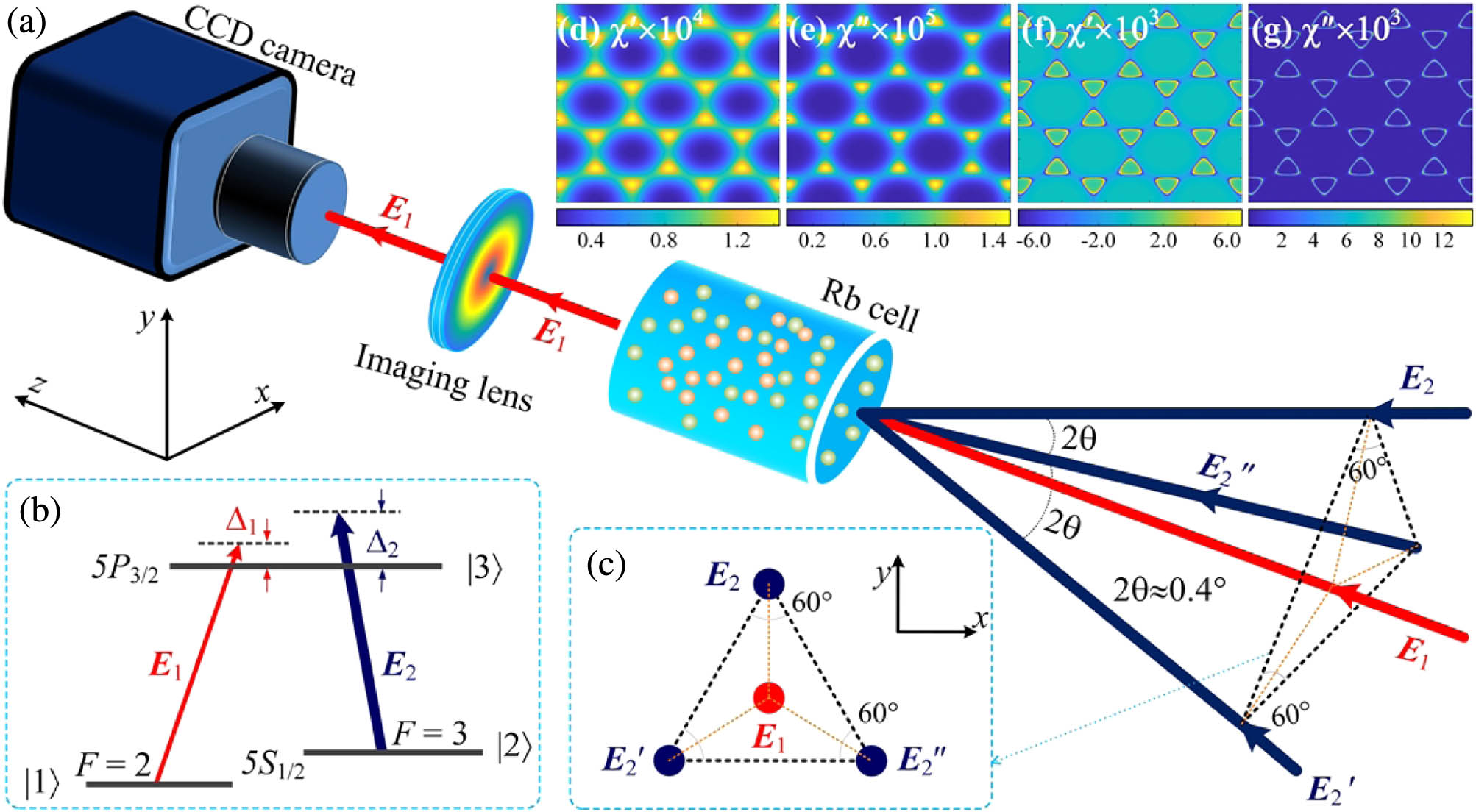
Fig. 1. (a) Experimental setup. Three coupling beams, E 2 E 2 ′ E 2 ′ ′ E c θ ≈ 0.4 deg x − y Δ 1 = − 60 MHz Δ 1 = − 110 MHz Δ 2 = − 100 MHz
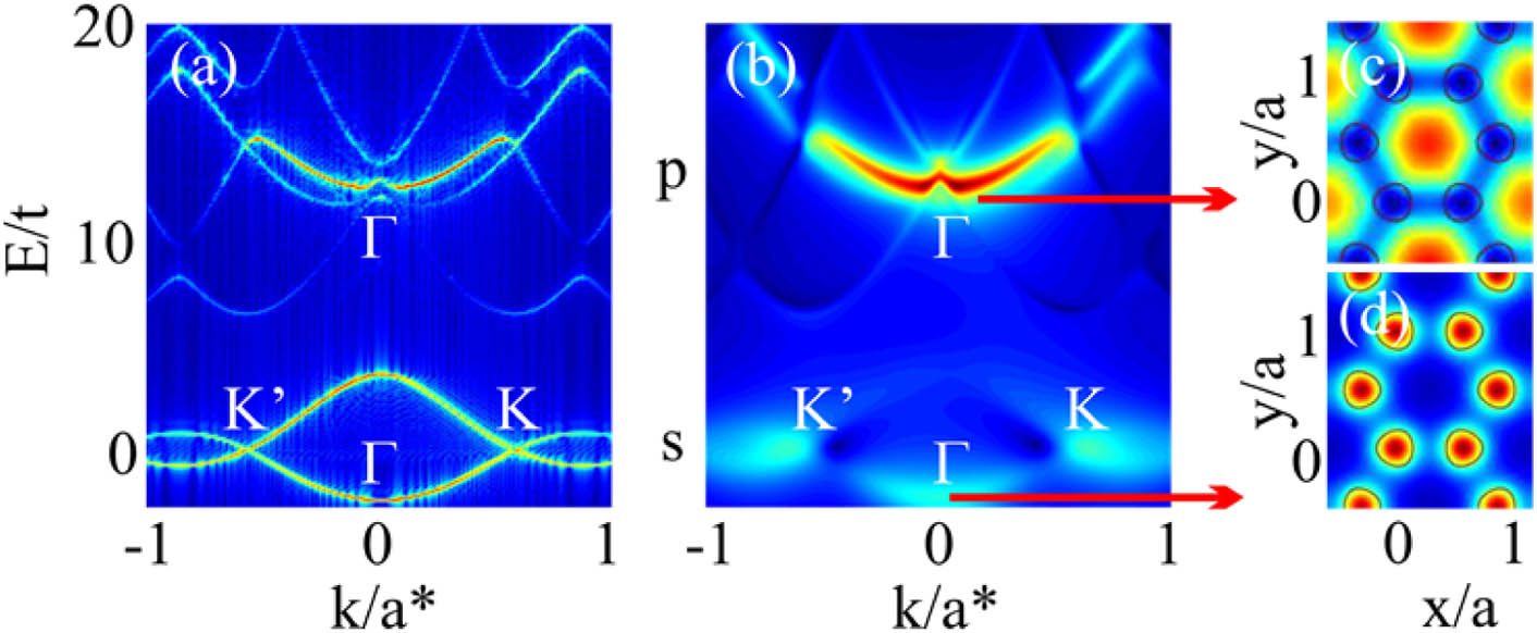
Fig. 2. Numerical simulations of a complex honeycomb photonic lattice. (a) Dispersion in the Hermitian case showing the lowest bands (s and mixed p / d Γ p / d Γ s p / d a a *
Fig. 3. Output probe patterns at different probe detunings. (a) Experimentally established coupling field; (b) observed discretized probe beam at different Δ 1 Δ 2 = − 100 MHz
Fig. 4. Observed self-imaging effect of the output probe beam at different probe detunings. (a) Δ 1 = − 90 MHz Δ 1 = − 110 MHz
Fig. 5. PT-symmetric-like transition measured by the symmetry factor as a function of the relative non-Hermiticity controlled by the detuning; black solid line, square root scaling; black dots, numerical simulations; red dots, experiment (error bars indicate the uncertainty).

Set citation alerts for the article
Please enter your email address
© Copyright 2018-2021 | Chinese Laser Press. All Rights Reserved 沪ICP备15018463号-20