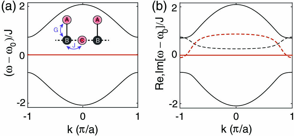
Fig. 1. (a) Band structure of a Hermitian Lieb lattice. The flat band is shown by the thick line. Inset: schematic of the Lieb lattice, where G (solid lines) is 3/4 of J (dashed lines). Partially transparent dots show the spatial profile of the compact Wannier function. (b) Same as (a) but with gain and loss modulation γA=1, γB=0.5, γC=−0.1. Dashed lines show the imaginary parts of the band structure, and those of the two dispersive bands are the same (given by the thin dashed line) due to the relation ωl(k)=−ωm*(k)(l≠m) imposed by NHPH symmetry.

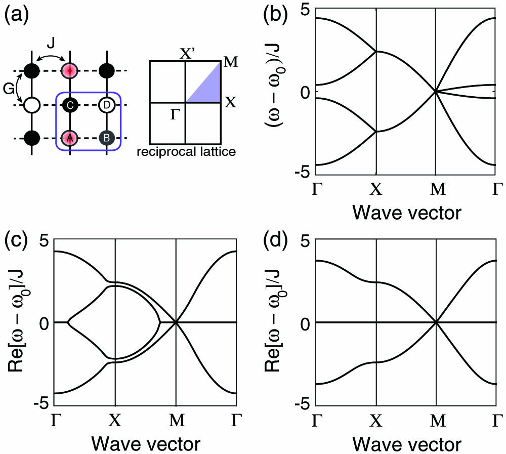
Fig. 2. Band structure of a 2D rectangular lattice with loss introduced to the A sites. (a) Schematics of the rectangular lattice and its reciprocal lattice. The unit cell is highlighted by the rounded box. G=1.2J>0. (b)–(d) Real part of the band structure when γA/J=0,−2,−4.8.

Fig. 3. Same as Fig. 2 but plotted in three dimensions with G=0.8J>0 and γA/J=−3.2 in (a) and −4 in (b).

Fig. 4. Band structure of the 2D square lattice shown in Fig. 2(a) but with a detuning ΔA=2J and γA/J=−4.8 in (a) and −20 in (b). The effectively Hermitian Lieb lattice in (b) and its band structure are shown in (c) and (d).

Fig. 5. Persisting and nonpersisting Hermitian flat bands. (a) Band structure of a Hermitian quasi-1D edge-centered square lattice. Inset: G (solid lines) =J (dashed lines). Partially transparent dots show the spatial profile of the compact Wannier function. (b) Same as (a) but with γA,B,D,E=0.5,γC=1. Again the imaginary parts (dashed lines) of the dispersive bands are identical pairwise due to NHPH symmetry. (c), (d) Same as (a), (b) but for a saw lattice with γA=0,γB=2. Inset in (c): G (solid lines) =2J (dashed lines).

Fig. 6. Persisting flat band in a 2D non-Hermitian Lieb lattice with G=1.2J>0. γB,C,D=−0.78,−0.71,0.32 in (a) and −2.1,−0.3,3.3 in (b).

Fig. 7. (a, b) Two compact Wannier functions (partially transparent dots) for the cross-stitched lattice shown. Couplings are represented by dashed lines (J), dash–dotted lines (J*), and solid lines (G). Gain (iγ) and loss (−iγ) are introduced to B and A sites, respectively. Here, G=|J|, Arg[J]=0.3≡θ/2, and γ=−G/sin θ in (a) and −G sin θ in (b). (c,d) Band structure of this cross-stitched lattice for the values of γ in (a) and (b). The flat bands result from the compact Wannier functions in (a) and (b).

Fig. 8. Polynomial power dependence for a localized initial excitation in an EP3 flat band. The excitation of (a) a Wannier function in a single unit cell, (b) a C site, and (c) an A site are shown by the red arrows. Note the different scales of the vertical axis in these three panels, even though the initial amplitudes of the excitation all equal 1. (d) Fixed amplitude |Ψ(C)|=1 at the excitation site in (b) (solid line) and linearly increasing amplitude |Ψ(A)| next to it (dashed line). (e) Quadratically increasing amplitude |Ψ(A)| at the excitation site in (c) (dotted line) and linearly increasing amplitude |Ψ(C)| next to it (dashed line).

Fig. 9. Relation between the three general approaches to construct a non-Hermitian flat band.