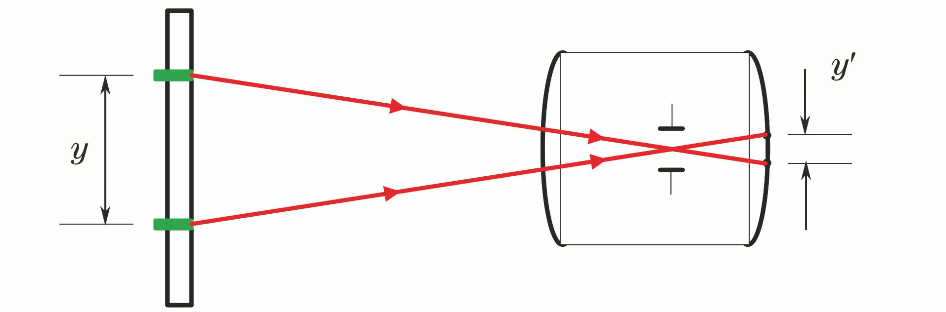
Fig. 1. Schematic of magnification measurement

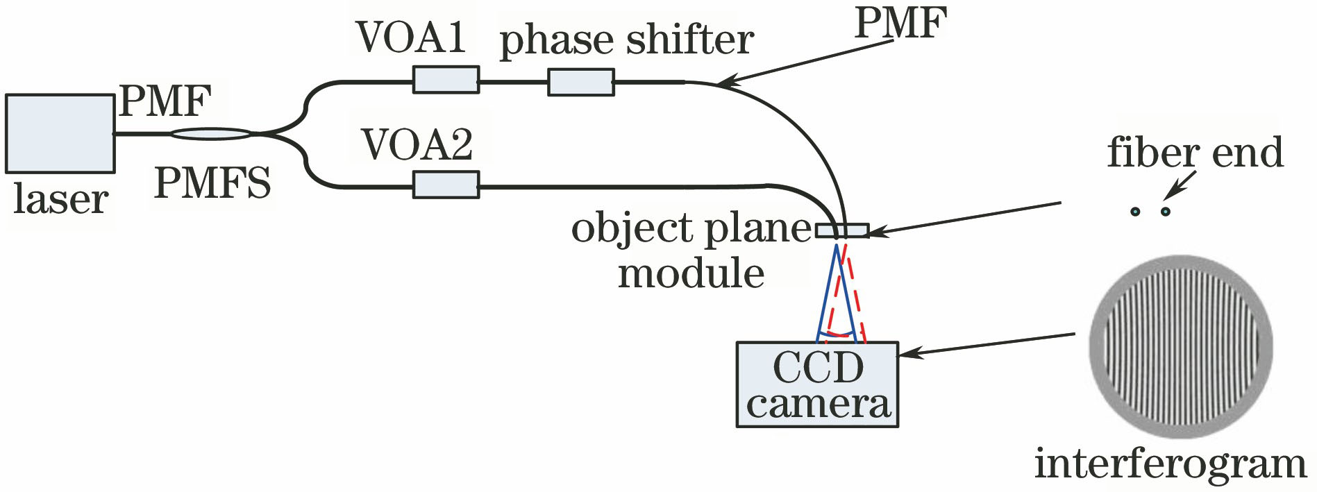
Fig. 2. Schematic diagram of object plane fibers spacing measurement system

Fig. 3. Mathematical model of fiber spacing measurement

Fig. 4. Wavefront and its Zernike coefficient obtained from ideal and non-ideal conditions. (a) Ideal wavefront; (b) ideal wavefront (without tilt); (c) Zernike coefficient of ideal wavefront; (d) non-ideal wavefront; (e) non-ideal wavefront (without tilt); (f) Zernike coefficient of non-ideal wavefront

Fig. 5. Quantitative relationship among point source separation distance, spatial location parameter of the CCD camera, and the Zernike polynomial coefficient. (a) Quantitative relationship between point source spacing and Z2 term coefficient; (b) quantitative relationship between vertical distance and Z7 term coefficient; (c) quantitative relationship between CCD rotation angle and Z2 term coefficient; (d) quantitative relationship between CCD rotation angle and Z3 term coefficient; (e) quantitative re

Fig. 6. Flow chart of fiber spacing measurement algorithm

Fig. 7. Schematic diagram of image plane fibers’ imaging points separation distance measurement system

Fig. 8. Spot center recognition results. (a),(b) Object location results; (c),(d) image location results

Fig. 9. Experimental wavefront and its Zernike coefficient values. (a) Object plane wavefront; (b) object plane wavefront (without tilt term); (c) Zernike coefficient of object plane wavefront; (d) image plane wavefront; (e) image plane wavefront (without tilt term); (f) Zernike coefficient of image plane wavefront

Fig. 10. Measurement repeatability of Zernike polynomial coefficient. (a) Object plane measurement result; (b) image plane measurement result

Table 1. Error requirement of fiber spacing measurement

Table 2. Settings of simulation conditions

Table 3. Initial parameter setting of iterative calculation

Table 4. Quantitative relationship among two fibers separation distance, spatial position parameters of the CCD camera, and the Zernike polynomial coefficient, and its calculation formula

Table 5. Simulation results of the effectiveness of the method for measuring the separation distance between two fibers

Table 6. Iterative calculation results of object plane separation distance between fibers

Table 7. Iterative calculation results of image plane separation distance between fiber image points