This paper presents a method to design a monolithic complete-light modulator (MCLM) that fully controls the amplitude, phase, and polarization of incident light. The MCLM is made of birefringent materials that provide different refractive indices to orthogonal eigen-polarizations, the ordinary and extraordinary states. We propose an optimization method to calculate the two relief depth distributions for the two eigen-polarizations. Also, a merging algorithm is proposed to combine the two relief depth distributions into one. The corresponding simulations were carried out in this work and the desired light distribution, including information on amplitude, phase, and four polarization states, was obtained when a laser beam passed through a 16-depth-level micro-structure whose feature size is 8 μm. The structure was fabricated by common photolithography. An experimental optical system was also set up to test the optical effects and performances of the MCLM. The experimental performance of the MCLM agrees with the simulation results, which verifies the validity of the algorithms we propose in this paper.
1. INTRODUCTION
A light wave contains multi-dimensional parameters: amplitude, phase, and polarization. Optical modulation technologies can be used to modulate these parameters to obtain desired optical effects, which have numerous practical applications, such as particle acceleration [1–5], laser fabrication [6,7], beam shaping [8–14], and holographic projection [15–24]. At present, most light field control techniques realize only partial control of the parameters of the incident light field. However, many experts and scholars have found that there are potential applications for a complete light control technique that can simultaneously control the amplitude, phase, and polarization of incident beams. For example, this technique can be used to structure the profiles of vector fields for special purposes, such as enabling a light beam to exert force and torque on illuminated objects [25,26]. The most attractive aspect of this technique is that it can be used to enhance the longitudinal component field [27] to obtain an optical needle field [28] or focus field [29], making it useful for particle capture and particle manipulation [30–32].
Davis et al.[33] designed polarization-multiplexed diffractive optical elements (DOEs) by using two cascaded liquid-crystal displays (LCDs). The first LCD encoded the two multiplexed phase-only DOEs. The second LCD acted as a pixelated polarization rotator to change the polarization state for each of these two DOEs. This approach was able to fully control all the parameters of the spatial distributions of an optical field. However, its optical system is difficult to align precisely. Plewicki et al.[34,35] proposed a method that can independently manipulate over the major axis orientation and the axis ratio of the polarization ellipse by integrating a shaper setup in both arms of a Mach–Zehnder interferometer and rotating the polarization by 90° in one of the arms before overlaying the beams. Moreno et al.[36] used a single transmissive spatial light modulator (SLM) to generate complex light fields. They divided an SLM into two regions, using the dual modulation of two transmissive subsystems to completely control the incident beam. Han et al.[37] proposed a cascaded modulation method that divided two reflective SLMs into four regions to form four reflective subsystems. This method generated various optical fields containing amplitude, phase, and polarization modulations. Chen et al.[38] and Liu et al.[39] designed different methods to generate two orthogonal complex fields. These two complex amplitude distributions generated desired light fields by coaxial superposition. The former used a phase-only SLM based on a system, while the latter divided a phase-type SLM into two regions, which respectively control the ordinary () ray and extraordinary () ray of the incident light. All of the above methods were based on SLMs to achieve full control of all parameters of incident light. It has to be acknowledged that these methods have great flexibility in light field modulation, but have the common disadvantages of complex systems and relatively high cost. Wang et al.[40] obtained a high-purity optical needle field by fabricating slot antennas on a metasurface structure. Each slot antenna can be regarded as a linear polarizer to fully control the light field. The system is greatly simplified, but in order to obtain the metasurface structure, the manufacturing cost is extremely high.
Our group previously designed a polarization multiplexing phase slice [41], which realized polarization multiplexing imaging on a single yttrium vanadate substrate (). In this manuscript, we report further developments of the modulation technique of a monolithic complete-light modulator (MCLM) and the design method for an MCLM that can yield a complex light field containing amplitude, phase, and polarization modulation. All parameters of the incident beam can be modulated without any other optical element except one MCLM. The system is simple and stable with little external interference and relatively low fabrication cost. This manuscript is organized with six sections. After this introduction, Section 2 demonstrates the principle of how to design the MCLM. Section 3 describes the design process about calculating the relief distribution of the MCLM. Section 4 shows the simulation result. In Section 5, we show the experimental results, which largely coincide with the simulation results. Section 6 is the summary.
2. PRINCIPLE
The design process of an MCLM includes the following three major steps. First, the desired light field containing amplitude, phase, and polarization information can be decomposed into two orthogonal components of o-ray and e-ray light fields and according to the Jones calculus. Second, a modified Gerchberg–Saxton (GS) algorithm [42] with both amplitude and phase limits is profiled to obtain two pure phase distributions and , which can be used to generate the phases of and . Third, by adopting point-by-point calculation, we can obtain a single relief depth distribution of birefringent material, which can obtain two phase delay distributions and of o- and e-ray light propagating in the birefringent material. The aim is to find an appropriate depth distribution of birefringent material that minimizes the error between and (). After searching for a suitable , the relief depth distribution of the MCLM can be obtained by quantizing to 16 depth levels.
When the incident light containing equal o-ray and e-ray light (i.e., linearly polarized light with a polarization orientation of 45° relative to the o-ray and e-ray axes of a birefringent material) passes through the MCLM, the o-ray and e-ray can simultaneously be modulated to generate and . The vector superposition of the two components generates the desired light field distribution .
3. DESIGN PROCESS
In the design process, the following parts should be considered carefully to obtain the depth distribution , which includes how to decompose the desired optical field into components of two orthogonally polarized complex light fields of proper amplitudes, how to retrieve two pure phase distributions of the two light fields by the modified GS algorithm, and how to obtain the relief depth distribution of birefringent material that can satisfy two phase distributions. The above three parts will be described in detail below.
A. Decomposition of the Desired Light Field
According to the Jones calculus, the desired light field containing complex information can be expressed as Equation (1) can be divided into two equations: in Eq. (1) stands for the desired light field, which can be regarded as the vector superposition of two orthogonal components of complex light fields and in Eq. (2). and are the common phase and phase difference of and , respectively. determines the polarization state distribution of desired field, and represents the polarization orientation.
An example of a desired light field of four regions containing amplitude, phase, and polarization is shown in Fig. 1.
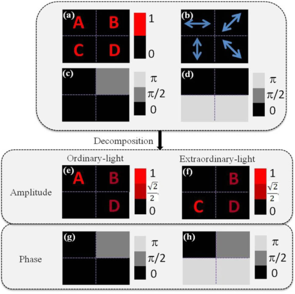
Figure 1.Example of a light field containing four regions as divided by the purple dotted lines. Distributions of the light field parameters are: (a) amplitude , (b) polarization , (c) common phase , (d) phase differience , (e) amplitude of , (f) amplitude of , (g) phase of , and (h) phase of .
Figure 1(a) shows , which contains patterns of different amplitude distributions of A, B, C, and D in different regions. Figure 1(b) shows that the polarization state distributions in four regions are linearly polarized, and the polarization orientation is indicated by four blue two-way arrows oriented at 0°, 45°, 90°, and 135°, respectively. Figure 1(c) represents the common phase , and Fig. 1(d) shows the phase difference .
In this example, the polarization state is linearly polarized, with in Fig. 1(b), the phase difference in Fig. 1(d); if in Fig. 1(b), the phase difference in Fig. 1(d); if or in Fig. 1(b), the phase difference in Fig. 1(d). Substituting , , , and into Eq. (2), the two components and can be obtained as By comparing Eqs. (2) and (3), we can obtain the amplitude and phase distributions of and , as shown in Figs. 1(e)–1(h).
Figures 1(e) and 1(f) represent the amplitude distributions and of and , respectively. Figure 1(e) shows that the amplitude of regions A, B, C, and D is equal to 1, , 0, and , respectively. Figure 1(f) shows that the amplitude of regions A, B, C, and D is equal to 0, , 1, and , respectively.
Figures 1(g) and 1(h) represent the phase distributions and of and , respectively. As can be seen from Eq. (2), the phase of is equal to the common phase . Meanwhile, the phase of is equal to .
B. Calculation of Phase Distributions
The common GS algorithm and most of the modified GS algorithm [43,44] can be used to calculate the desired light field only with amplitude distribution, while the phase distribution cannot be considered. However, in this paper, since and contain determinate amplitude distributions and phase distributions, it is necessary to optimize the calculation by using the modified GS algorithm for both amplitude and phase limitations. In the iterative process, the output plane is divided into the signal domain and the noise domain, as shown in Fig. 2. To avoid the influence of the center zero-order on the experimental results, the signal domain is placed at a position offset from the center of the output plane.
Figure 2.Flow chart of the modified GS algorithm with both amplitude and phase limits.
Taking as an example, the specific steps can be described as follows. The initial phase distribution of design phase plane is random value from 0 to , denoted as .
The process of modified GS algorithm is shown in Fig. 2. First, the amplitude of the design phase plane is replaced by 1 to obtain complex amplitude , . Then propagates from the design phase plane to the output plane, which generates a failed complex amplitude distribution . is the modified Fresnel-domain constraint function to correct the failed results, which can be expressed as where and are the amplitude distribution and phase distribution of , respectively. is the weight factor. and refer to the signal domain and the noise domain, respectively. Second, when the modified function propagates back to the design phase plane, the complex amplitude distribution will be generated. To obtain a phase-only distribution, we retain only the phase distribution , while the amplitude is eliminated. Finally, becomes the phase distribution at the beginning of the next iteration of the design phase plane.
During the iteration, we need to determine whether the failed result meets the error requirement, which can be represented by the root mean square error, as shown in Eq. (5). If so, the iteration is terminated and the pure phase distribution [i.e., ] becomes the output of the iteration; otherwise, the iteration continues. Meanwhile, can also be obtained by using the modified GS algorithm. where RMSE stands for the root mean square error of amplitude between the failed result and the desired result .
Adopting the proposed algorithm, and can be calculated. Then, and will be used to search the relief depth distribution of the MCLM.
C. Search of Relief Depth Distribution
According to the refractive indices and of the ray and ray propagating in birefringent material, the relief depth distributions and can be calculated by where is the refractive index of a light wave whose wavelength is , and is the relief depth of the DOE.
However, and have entirely different distributions. To simultaneously modulate and light by a single MCLM to obtain the two orthogonal components of the desired light field, it is necessary to optimize the two different relief depth distributions to a unique relief depth distribution .
The calculation process is as follows. Suppose the array size of the MCLM is , and the relief depth of the pixel on the MCLM is , where . Utilizing Eq. (6), the phase delays of for the and light can be calculated as and . Therefore, the phase errors between and () can be calculated as and . However, as we all know, due to the periodicity of the phase, it is difficult to calculate the actual phase error. Therefore, () is used here to characterize : where represents the remainder of divided by . We regard the square sum of and as the equivalent judgment equation of the total phase error: Obviously, as the changes, the errors also change. When is the smallest, a suitable can be found, which is the relief depth of the MCLM. In this paper, equal-interval search is adopted to calculate . Taking the e-ray as a reference, In Eq. (9), ( is an integer), where is also an integer used to determine search accuracy. Each search interval of is . Note that the larger is, the higher the search accuracy is, but the longer the calculation time will be. In general, we take . Substituting into Eq. (9), we can obtain values of , which are . Substituting the values into Eq. (7), and then utilizing Eq. (8), we can find a suitable that minimizes .
Each pixel is optimized in the same manner, and the final relief depth distribution can be obtained. Theoretically, if the value range of is not limited (), it is certain that an appropriate can be found to make . However, it is necessary to consider the actual processing situation. In reality, if the depth is too shallow, it is difficult to find a suitable , while if the depth is too deep, it is not conducive to machining. Meanwhile, if the depth falls outside a certain depth range, the quantized result will become worse. Therefore, when determining the value range of or the value of , it is necessary to comprehensively consider the above situations.
In this paper, to simplify the calculation, the search range of depth is chosen as an integer multiple of , which provides a phase modulation of integer multiple of for the e ray [see Eq. (6)]. Since the maximum value of in Eq. (9) is , for satisfying the above condition, it requires to be an integral multiple of . First, let . The optimal depth distribution is calculated by the equal-interval search algorithm, which is quantized to a 16-level structure. Two orthogonal complex fields will be calculated by diffraction calculation for the o and e rays, which will be substituted into Eq. (5) for calculating the two root mean square errors between the two calculated complex fields and the desired orthogonal complex fields, respectively. Second, in the same manner, multiple optimized depth distributions respectively corresponding to will be searched, and multigroup root mean square errors can be calculated. Finally, according to the criterion of minimizing the sum of root mean square errors, we determine that the 16-level relief depth distribution corresponding to is the most appropriate.
4. SIMULATION
To verify the correctness of the above algorithm, we took a desired light field, with its parameters as shown in Figs. 3(a)–3(d), to carry out the simulation, where Fig. 3(a) is the intensity distribution of the desired light field that was used to characterize the amplitude distribution . It is composed of four characters from the movie “Journey to the West.” Figure 3(b) represents the polarization state. The polarization state of each character is linear polarization, with , 45°, 90°, and 135°, as indicated by four blue arrows. Figure 3(c) shows that the common phase of the first two characters was equal to and the rest are equal to 0. Figure 3(d) shows that the phase difference of the last two characters is equal to and the rest are equal to 0.
Figure 3.Parameters of the light field in the four regions: (a) intensity , (b) linear polarization , 45°, 90° and 135°, (c) common phase , and (d) phase differience .
The wavelength of incident light was 632.8 nm. The birefringent material we chose was , which had a large birefringence with refractive indices and of 1.9929 and 2.2154, respectively. The array size used in the simulation is 1024 by 1024, with a pixel size of μμ. The imaging distance was 0.7 m. We have compiled the modified GS algorithm and relief depth search algorithm, and simulated the light field modulation effect of the MCLM by using the software MATLAB. The relief depth distribution of MCLM which has 16 levels is shown in Fig. 4. The deepest relief depth of the MCLM is 1.95 μm. The depth difference between adjacent levels is 0.13 μm.
Figure 4.Relief depth distribution of the MCLM that has 16 levels. The depth difference between adjacent levels is 0.13 μm.
The designed MCLM is examined through simulation using a polarization analyzer for incident light with equal amounts of the two orthogonal eigen-polarizations, and the resultant light field distributions are shown in Figs. 5(a)–5(e).
Figure 5.Simulation results: (a) without polarizer; with polarizer oriented at (b) 0°, (c) 45°, (d) 90°, and (e) 135°.
Figures 5(a)–5(e) represent the simulation result with 16 levels of quantization. Without a polarizer, all four characters appear as shown in Fig. 5(a). Moreover, the simulated intensity distribution is consistent with the original desired intensity distribution, which proves that the method can achieve the control of the amplitude of the incident light. Then, we simulated the case where a linear polarizer analyzer was added to detect the polarization state of the reconstructed light field. Figures 5(b)–5(e) simulated that when the linear polarizer analyzer was oriented at 0°, 45°, 90°, and 135°, the four characters appeared or disappeared in turn. For example, when the linear polarizer analyzer is oriented at 0°, the third character completely disappears [Fig. 5(b)]. This confirmed that the area where the third character is located has linearly polarized light with its polarization orientation at 90°. Therefore, it could be seen from Figs. 5(b)–5(e) that the light in the areas of each of the four characters is all linearly polarized with their polarization orientations at 0°, 45°, 90°, and 135°.
As can be seen from the simulation results, the modulation of amplitude and polarization by a single MCLM can be realized. Meanwhile, according to the description of Section 3.A, the determined polarization state indicates that the phase difference between the ray and the ray is determined. Therefore, the modulation of phase can also be achieved by the MCLM. Furthermore, this method can also be utilized to completely control a more complex light field.
5. PREPARATION AND EXPERIMENTAL RESULTS OF MCLM
To verify the above design method and the simulation results, the designed MCLM was fabricated and the optical effects were tested by experiments. Here, a photolithography technique was used to carry out the fabrication. As the designed MCLM was quanticized to 16 levels of depth, multiple exposure and etching processes were carried out. The fabrication process of the 16-level structure is illustrated in Fig. 6.
Figure 6.Fabrication process of the MCLM: (a) the first etching with etching depth of 130 nm, (b) the second etching with etching depth of 260 nm, (c) the third etching with etching depth of 520 nm, and (d) the fourth etching with etching depth of 1024 nm.
Four masks used in the process are shown in Fig. 7. The masks were used to carry out the exposure one by one to form the 16-level structure. Also, etching processes were carried out four times to transfer the structure into the birefringent crystal material. The etching depths in the four etching processes were 130, 260, 520, and 1040 nm. We ranked the four masks according to the etching depth from shallow to deep. The area within the blue dashed line represents the graphic area of the masks, as shown in Fig. 7(a). As can be seen from the structure observed by microscope of the four masks, the graphic area was divided into two parts, which were black and white. During the exposure process, the black and white parts determined whether light could pass through the mask.
Figure 7.Four masks used in the MCLM fabrication process: (a) mask one, (b) mask two, (c) mask three, and (d) mask four.
The photoresist material AZ9260 was used to carry out the exposure. The photoresist was spin-coated on the crystal substrate with rotation speed of 5000 rad/min. Process parameters of coating time, prebake temperature, prebake time, and resist thickness were 30 s, 100°C, 10 min, and 3 μm, respectively. An exposure system was employed to perform the exposure process, with a illumination light source that is a Hg lamp with a central wavelength of 365 nm. The total exposure time was 20 s. Process parameters of development, after-bake temperature, and after-bake time were 30 s, 120 °C, and 60 min, respectively. Ion beam etching was carried out to transfer the structure into the substrate. The etching times in four etching processes were 15, 30, 60, and 120 min. The resulting average depths of the four etchings were 141, 240, 539, and 1050 nm, respectively. The practical and theoretical depth errors were , , , and , respectively. The pictures of the obtained elements are shown in Fig. 8. Figure 8(a) shows the photograph of the fabricated MCLM and Fig. 8(b) shows the photo taken by microscope, from which we can see the structure detail.
Figure 8.(a) Fabricated MCLM. (b) Structure of the MCLM observed under microscope.
The experimental setup and light beam path were built to test the MCLM, as shown in Fig. 9. The laser beam first propagated through a polarizer oriented at 45° in order to obtain incident linearly polarized light containing equal-amplitude o-ray and e-ray light. Then, the obtained linear polarized light passed through MCLM to produce the desired light field, of which polarization state was detected by a linear polarizer analyzer. The distance from the CCD to the location of the MCLM was 0.7 m, which was the same as in the simulation process.
Figure 9.Experimental setup and light beam path for testing the MCLM performance.
The desired intensity pattern was received by a CCD (Fig. 10). Figure 10(a) shows the reconstructed light field, of which the intensity distribution was consistent with the desired light field. When there was no linear polarizer analyzer, four characters appeared in the light field. By using the polarizer analyzer to detect the polarization state of the desired light field, we have obtained the patterns shown in Figs. 10(b)–10(e). When the linear polarizer analyzer was oriented at 0°, 45°, 90°, and 135°, the four characters disappeared one after another. As shown in Fig. 10(b), the third character completely disappeared when the polarizer analyzer was oriented at 0°. This indicated that the area where the third person was located was 90° linearly polarized. Detecting by the linear polarizer analyzer, it was easy to see that the polarized orientations of the four characters are 0°, 45°, 90°, and 135°.
Figure 10.Experimental results. The desired intensity pattern is received by a CCD. (a) No polarizer analyzer. In (b)–(e), the polarizer analyzer was oriented at 0°, 45°, 90°, and 135°, respectively.
Meanwhile, it could be seen from the experimental results that the light field generated by the MCLM was basically consistent with the theoretical simulation results shown in Figs. 5(a)–5(e), with only a few deviations caused by residual manufacturing errors in the MCLM. It could be considered that the experimental results were in great agreement with the simulation results. Therefore, by utilizing only one MCLM, we have successfully controlled the phase, amplitude, and polarization of incident light.
6. CONCLUSION
In this paper, we have proposed a new type of optical modulation element called MCLM. The simulation and experimental results have shown that the MCLM successfully realizes complete control of incident light amplitude, phase, and polarization to obtain a tunable complex light field. The method proposed in this paper can achieve any optical response controlled by only one single MCLM component. The system is simple and stable with little external interference. Moreover, it is expected to be used in the areas of optical fabrication and light trapping.
[43] R. W. Gerchberg, W. O. Saxton. A practical algorithm for the determination of phase from image and diffraction plane pictures. Optik, 35, 1-6(1972).