Lan Yu, Yu Wang, Yang Wang, Kequn Zhuo, Min Liu, G. Ulrich Nienhaus, Peng Gao, "Two-beam phase correlation spectroscopy: a label-free holographic method to quantify particle flow in biofluids," Photonics Res. 11, 757 (2023)
Copy Citation Text
We introduce two-beam phase correlation spectroscopy () as a label-free technique to measure the dynamics of flowing particles; e.g., in vitro or in vivo blood flow. combines phase imaging with correlation spectroscopy, using the intrinsic refractive index contrast of particles against the fluid background in correlation analysis. This method starts with the acquisition of a time series of phase images of flowing particles using partially coherent point-diffraction digital holographic microscopy. Then, phase fluctuations from two selected circular regions in the image series are correlated to determine the concentration and flow velocity of the particles by fitting pair correlation curves with a physical model. is a facile procedure when using a microfluidic channel, as shown by the measurements on flowing yeast microparticles, polymethyl methacrylate microparticles, and diluted rat blood. In the latter experiment, the concentration and average diameter of rat blood cells were determined to be μ and μ, respectively. We further analyzed the flow of mainly red blood cells in the tail vessels of live zebrafish embryos. Arterial and venous flow velocities were measured as μ and μ, respectively. We envision that our technique will find applications in imaging transparent organisms and other areas of the life sciences and biomedicine.
1. INTRODUCTION
To characterize the transport of nanoscopic and microscopic particles (e.g., active movement of vesicles along microtubules in cells or the flow of blood cells in vessels), it is important to understand many biological processes [1,2]. A variety of techniques have been proposed to quantify the dynamics of particle flow, including particle image velocimetry (PIV) [3,4] and optical Doppler tomography (ODT) [5–8]. PIV, which involves continuous imaging of many small tracer particles to analyze the speed and direction of the flow pattern, is limited in temporal resolution. In ODT, the flow velocity at a specified location in the conduit is determined by measuring the interference between the backscattered light from a sample and a reference arm and analyzing the Doppler frequency shift. ODT is a noninvasive, noncontact optical technique; currently the ODT time resolution is mainly limited by the necessity to record hundreds of holograms for each swept wavelength [9]. Another major difficulty for Doppler flow imaging is to separate the Doppler flow signal from background noise; e.g., induced by tissue micromotion and heterogeneity [7]. Fluorescence correlation spectroscopy (FCS) [10–14] has also proven to be a valuable tool for the quantitative assessment of particle flow. In standard FCS experiments, a laser beam is focused into a sample to create a tiny observation volume of , from which the fluorescence emitted by particles moving through the volume is registered as a function of time [15]. Time autocorrelation analysis of the intensity yields quantitative information about diffusion and flow. Two-beam FCS [16] has proven to be a valuable tool to determine flow parameters, including both flow velocity and flow direction using cross-correlation. Compared to single-beam FCS, two-beam FCS can capture greater flow velocities and provides information about the flow direction [16]. However, both FCS and two-beam FCS require either intrinsically fluorescent particles, or particles labeled with fluorescent moieties. The unavoidable photobleaching limits its application and calls for techniques that do not rely on fluorescence.
The refractive index (RI) is an intrinsic optical parameter related to the electrical permittivity of the material. The RIs of biological particles, subcellular organelles, or cells differ from their (usually aqueous based) surrounding biofluid; therefore, the RI can provide the necessary contrast against the background. The RI of subcellular organelles can be measured with high accuracy using quantitative phase microscopy (QPM) [17–22]. Cheong et al. [23] employed label-free holographic (inline holography) flow cytometry to study avidin binding to biotinylated polystyrene spheres. Min et al. [24] combined off-axis digital holographic microscopy (DHM) with flow cytometry to determine the features of different cells. Merola used tomographic flow cytometry to characterize the flow of red blood cells and diatom algae in a microfluidic channel [25]. All these methods exploit phase information to create the necessary contrast. Notably, the measurable flow speed is limited due to the particle trajectory-based analysis.
Here, we present two-beam phase correlation spectroscopy (2B-ΦCS), a label-free approach to quantify particle flow, such as in vivo blood flow or particle flow through a standard microfluidic chip [26–28]. In , phase fluctuation time traces are acquired by quantitative phase imaging, and correlation analysis yields information on the concentration and velocity of flowing particles. overcomes photobleaching and phototoxicity issues inherent in fluorescence-based approaches, and thus can be widely applied in many fields, including biomedicine.
Sign up for Photonics Research TOC. Get the latest issue of Photonics Research delivered right to you!Sign up now
2. METHODS AND RESULTS
A. Principle of
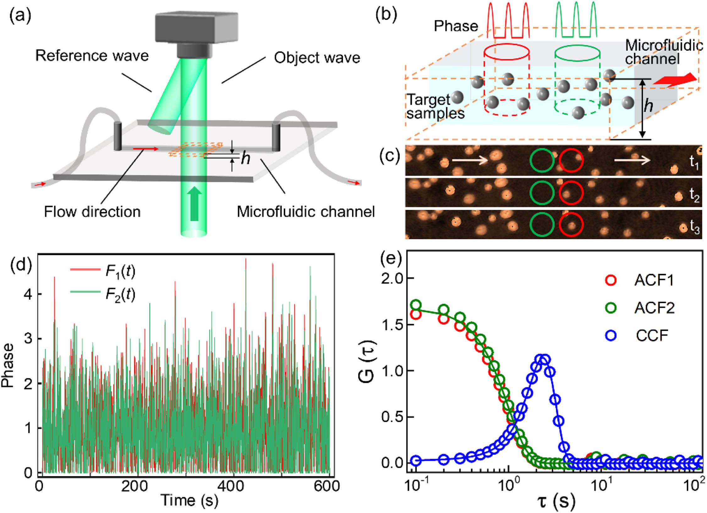
To implement with a microfluidic chip [Fig. 1(a)], we drove a fluid containing particles through a channel with a width of 1 mm and a height of 100 μm, thus avoiding defocus [Fig. 1(b)]. The sample was imaged (perpendicular to the flow direction) by partially coherent point-diffraction digital holographic microscopy (PC-pDHM) using a objective. With its common path configuration, PC-pDHM has an ultrahigh phase stability against external disturbances and a high sensitivity to refractive index changes in the sample. The illumination beam propagated vertically through the channel. The transmission image was magnified by a microscope system and recorded by a camera after interfering with a reference wave. A sequence of holograms was recorded by a camera (DMK33UX174, The Imaging Source, LLC, Charlotte, NC, USA) at a rate up to , limiting the time resolution to ca. 6 ms. Phase images are reconstructed using the conventional off-axis hologram reconstruction algorithm [Fig. 1(c)].
Figure 1.Principle of . (a) Sketch of the microfluidic channel (width 1 mm, height μ) illuminated by a perpendicular light beam. The sample flowing through the microchannel is monitored by phase imaging. (b) Enlarged region marked by the dashed orange box in (a). Phase information is extracted from two illuminated regions indicated by red and green cylinders. (c) Recorded phase images at , , . The red and green circles correspond to the observation regions in (b). The white arrows indicate the flow direction. (d) and are the corresponding phase-time traces. (e) ACFs and CCF curves calculated from the phase-time traces.
Two circular regions of interest (ROIs), shown by the red and green circles in Fig. 1(c), were selected in the phase image series. Two phase-time traces, and , were calculated by integrating the phases of all pixels within the red and green ROIs, respectively, for every time point, [Fig. 1(d)]. From the two time traces, two autocorrelation functions (ACFs) and a cross-correlation function (CCF) were calculated [Fig. 1(e)] as where represents the ACFs of the two traces, with time lag and trace index ; and is the CCF of the two traces. Angular brackets indicate averaging over all the pairs of phase values within the recorded data set.
In close analogy to FCS [16,29], the amplitude of is equal to the reciprocal of the mean number of the particles in the two observation volumes [Fig. 1(b)]. The width of represents the average residence time of a particle in the observation volume, whereas the peak of gives the time a particle takes to move from the first to the second region. For diffusional motion superimposed with a constant velocity flow, the ACFs and CCF can be globally fitted with the model functions
Here, is the correlation time of the particle flow (i.e., the average time a particle takes to transit the circular ROI with radius ), and is the spatial displacement between the centers of two ROIs. Note that the fitting model is equivalent to the two-beam FCS [16] for flow analysis [29,30], with the particle phase as the observable instead of the fluorescence intensity. The 2D free diffusion of the measured species was captured by the term , with the diffusional correlation time . By using nonlinear least-squares fits of Eq. (2) to the experimental and curves, the parameters could be determined. The concentration of the particles was calculated from using . Furthermore, the average flow velocity of the particles was determined using . For typical biofluid applications, such as fluid flow in biological vessels, is one or two orders of magnitude greater than , so we neglected diffusion in the analyses of the different applications presented below.
In general, can be applied to measure flow velocities spanning a broad range by adjusting the parameter because a larger is obviously more suitable for larger flow velocities. Our present time resolution of 6 ms is sufficient to monitor the fluid flow with speeds in the range of μ (see Section 2.E), selecting two ROIs with suitable radii and mutual displacement.
B. Comparison of Phase and Amplitude Correlations
To demonstrate the enormous sensitivity enhancement of phase over intensity correlation analysis, we performed time correlation analysis using either the amplitude or the phase as the observable to measure the particle flow. To this end, 5 μm diameter yeast cells (Angel Yeast Co., Ltd., Yichang, China) were diluted in phosphate-buffered saline (PBS) solution to a concentration of (Section 3.D). The solution was pumped through the microfluidic channel sandwiched between two cover slips and imaged by PC-pDHM for 200 s at a frame rate of . Amplitude and phase images were reconstructed from all 6000 images, shown three times in Figs. 2(a) and 2(b), respectively. Two circular regions, with radii μ and a mutual displacement μ along the flow direction were selected for the amplitude and phase image series, and amplitudes and phases within the circular regions were integrated to form two time traces. From the resulting amplitude-time and phase-time traces, ACFs and CCF were calculated with Eq. (1) and fitted with Eq. (2). This process was performed with 10 groups of amplitude and phase image sequences to obtain the mean ACFs and CCF shown in Figs. 2(c) and 2(d), respectively. Obviously, the phase images have much higher contrast than the amplitude images; therefore, they have a much-enhanced SNR. The fit of the ACFs and CCF curves in Fig. 2(d) with the model in Eq. (2) yielded μ and μ.
Figure 2.Comparison of amplitude- and phase-based correlation analysis. (a), (b) Amplitude and phase images, respectively, of yeast solutions, acquired at (top to bottom) , 0.5 s, and 0.9 s (Visualization 1). The white arrows in () and () show the flow direction in the yeast solution. (c), (d) ACFs and CCF calculated from the amplitude and phase image sequences, respectively. Symbols and error bars represent means and standard deviations, respectively, calculated from a set of 10 independent measurements.
C. Analysis of Velocity and Concentration of PMMA Microspheres
We further tested for measuring the flow velocity of polymethyl methacrylate (PMMA, KM-5050, diameter 5 μm, DG KM New Material Co., Ltd., Dongguan, China) beads dissolved in an aqueous (PBS) solution. The solution flowed through a microfluidic channel with an electrical pump at three different speeds. For each of the three measurements, we took 6000 DHM holograms in 200 s. The procedures and ROI setting were the same as in Section 2.B. As expected, the peak of the CCF shifts to shorter times with an increase in the flow speed [Fig. 3(a)]. The global fit of and with Eq. (2) further revealed μ, μ, and μ for the three flow speeds. The results agreed within the error found by PIV-based analysis, yielding μ, μ, and μ, but had markedly smaller uncertainties [Fig. 3(b)]. Note that in PIV-based analysis 30 beads were randomly selected for velocity determination.
Figure 3.Measurement of three different flow speeds of PMMA microspheres using . (a) Normalized curves (flow speeds are given in the legend); symbols and error bars: mean standard deviations from 10 independent experiments. (b) Histogram comparing flow speeds from and PIV; data1, data2, and data3 refer to the sets of experiments at the three different flow speeds. Error bars are shown as obtained from the fit () and as standard deviations from the PIV analysis of 30 beads equally distributed in 10 independent experiments (i.e., three beads were selected from each data set).
The large error here was mainly due to the parabolic flow velocity of the selected particles with respect to their distance to the surfaces of the channel (Poiseuille’s law). Thus, had the merit of a simpler analysis and yielded more reliable results since more particles were included. However, the measurement yielded the flow velocity averaged over the velocity distribution of all registered individual particles.
We further explored the capability of to determine the concentration of flowing particles. The PMMA particles were prepared with three concentrations: μ, μ, and μ that were determined by simply counting the particle number in the field of view and dividing it by the volume. Figure 4(a) shows the two (essentially identical) ACFs and CCF for three different concentrations.
Figure 4.Measurement of particle concentrations of PMMA microspheres using . (a) Three sets of correlation curves of PMMA microspheres with different concentrations (given in the legend). (b) Linear relationship between the results obtained by , and by simply counting PMMA particles in the volume. The open symbols indicate the individual data points of different concentrations, while the solid symbols indicate the mean of the data points with the same color.
It is obvious that the amplitudes decrease with an increase in the PMMA concentration. The fit of the correlation curves with Eq. (2) gives the concentrations as μ (blue), μ (green), and μ (red), which was in excellent agreement with the counting results.
D. Determination of Red Blood Cell Concentration and Diameter
To measure the concentration of red blood cells (RBCs) in vitro, blood was drawn from the rat [Sprague Dawley (SD) rat, Air Force Medical University, Xi’an, China] and diluted with PBS at a volume ratio of 1:100. The solution was measured, as illustrated in Fig. 5(a), using the same procedure as in Section 2.C. Phase images were reconstructed from the recorded holograms; a few selected ones are shown in Fig. 5(b). We selected two circular ROIs with μ and μ. ACFs and CCF were calculated and fitted with Eq. (2) to obtain the concentration of RBCs in the solution. The measurement was repeated 35 times; for each measurement, eight sets of regions were selected for analysis to yield 280 independent data points, which is shown as a histogram in Fig. 5(c). A Gaussian fit revealed that an average concentration of RBCs was μ ().
Figure 5.Analysis of the concentration and size of rat RBCs. (a) Workflow of in vitro measurement on rat blood. (b) Phase images of flowing RBCs at six different times. (c), (d) Histograms of (c) concentration and (d) diameter measurements.
Furthermore, the RBC diameter could be assessed with the phase image correlation approach mentioned in Section 3. A phase image was transformed into a time trace , and the ACF of was calculated with the first equation in Eq. (1). The fit of the ACF with Eq. (3) (Section 3) provided the average particle diameter. The measurement was repeated 30 times, and six phase images were selected from each measurement for the analysis to yield 180 data points which were compiled in a histogram [Fig. 5(d)], revealing an overall average diameter of μ (). Notably, the measured concentration and radius agreed well with the reported concentration μ [30] and diameter range (μ) of rat RBCs [31].
E. Measuring Blood Flow in a Live Zebrafish Embryo
The in vivo characterization of blood flow is important in both clinical diagnosis and biomedical research. In this section, was used to monitor blood flow in live zebrafish embryos, as depicted in Fig. 6(a). Live embryos (three to four days post fertilization) were anesthetized and imaged at a rate of . An exemplary phase image reconstructed from the PC-pDHM hologram series [Fig. 6(a), right hand side] shows RBCs in a vein (posterior cardinal vein, PCV) and an artery (dorsal aorta, DA) in phase contrast. For analysis, we again selected two circular regions, from which the phase values were extracted to form time traces. As an example, ACFs and CCF calculated from the DA data are shown in Fig. 6(b). The ACFs and CCF displayed artifacts within the time range of 0.1–0.5 s; i.e., the curves drop below zero. This was caused by the periodic acceleration of the blood due to the heartbeat. The global fit of the ACFs and CCF curves with the model in Eq. (2) revealed a flow speed in the artery of μ. Figure 6(c) shows the statistics on the flow velocities of RBCs in arteries (red square) and veins (gray square) characterized by on 15 zebrafish embryos, yielding average flow velocities of μ () in the DA and μ () in the PCV. Thus, blood flows roughly twice as fast in the DA as in the PCV. PIV-based analysis on the same phase images gave μ () for DAs and μ () for PCVs, showing agreement with within the error. The considerable spread of the mean over the population likely reflects (size) variations within the zebrafish ensemble [32]. This experiment demonstrates that can be applied to in vivo measurements of blood flow in live zebrafish.
Figure 6.In vivo measurement of blood flow velocities in an artery and a vein of a zebrafish embryo. (a) Schematic DHM setup for measurement on blood cell flow in zebrafish vessels (Visualization 2). The insets show the schematic diagram (top) and an enlarged image of the dorsal aorta (DA) and posterior cardinal vein (PCV). The arrows in the phase image show the blood flow directions in the two vessels. (b) ACFs (red and green) and CCF (blue) calculated with the phase values within two circular regions in the blood vessel. (c) Statistics on the velocities of blood flow in the artery and vein of zebrafish.
Partially coherent point-diffraction DHM (PC-pDHM) [35] was used to acquire quantitative phase images of all samples. The PC-pDHM used in our experiments is equipped with a microscope objective. The spatial resolution of the system was 0.8 μm upon illumination with 532 nm light. The off-axis hologram has and a carrier frequency of μ. Compared to conventional DHM, PC-pDHM has a common path configuration and is, therefore, robust against environmental disturbances. Furthermore, the use of partially coherent illumination endows PC-pDHM with a high SNR. For measurements, the samples, either the microfluidic chip or the live zebrafish embryo, were mounted on top of the objective of the PC-pDHM, and off-axis holograms were recorded sequentially in time. Both amplitude and phase images were reconstructed from the recorded holograms using an angular spectrum-based approach [35]. Notably, the defocus of the sample can be digitally compensated by propagating the reconstructed wave from the hologram plane to the image plane. analyses were performed on the phase image series using Eqs. (1) and (2).
B. Fabrication of Microfluidic Device
For on flowing particles and blood cells, a transparent microfluidic device was fabricated as follows. Two rectangular strips of double-sided adhesive tape were placed on a glass substrate ( microscope slide), leaving a 1 mm wide gap. A channel was formed by using a microscope cover glass as a top cover. The resulting channel had a depth of 100 μm (measured by confocal microscopy), which ensured that particles of various sizes could pass the channel and, furthermore, avoided defocus of particles in different layers during PC-pDHM imaging. Fluid inlet and outlet ports were made by drilling two holes (1.5 mm diameter, 30 mm apart) at the two ends of the channel and connecting them to microfluidic tubes with an inner diameter of 0.5 mm.
C. Radius Determination from a Single Phase Image
The radius of an RBC can be assessed from a single phase image using phase image correlation analysis [36], which also uses phase image sequences of the sample. In this method, a time trace is generated by rearranging the pixelated phase values in the phase image along a raster scanning pathway. From this sequence, the ACF of was calculated with the first equation in Eq. (1) and fitted with
Here, is the average particle radius, is the average particle number in the observation volume , and is the pixel size of the CCD camera. is an independent variable that represents the pixel displacement. This method yields the particle radius from a single-phase image; hence, it is fast.
D. Preparation of Yeast and PMMA Bead Solutions
Natural highly active dry yeast (diameter 5 μm, Angel Yeast Co., Ltd.) and PMMA microparticles (PMMA, KM-5050, diameter 5 μm, DG KM New Material Co., Ltd.) were used without further purification. A total of 30 mg of yeast was dissolved in 50 mL deionized water to generate 0.6 g/L concentration for the velocity measurements shown in Fig. 2. Similarly, PMMA microparticles were dissolved in deionized water to generate three different concentrations of 2, 3, and for the concentration measurements shown in Figs. 3 and 4. Both yeast and PMMA solutions were vortexed before the experiments to ensure monodispersity.
E. Rat Blood Preparation
Blood was freshly drawn from the rat and stored in an anticoagulation tube. Before the measurement, we diluted the rat blood a hundred fold with a PBS solution, filled it into a syringe, and pumped it through the microfluidic chamber at a constant rate for data acquisition.
F. Zebrafish Embryo Preparation
Live wild-type zebrafish embryos (strain AB, Shanghai FishBio Co., Ltd.) were cultured at 28°C (14 h in light and 10 h in the dark each day) for three or four days post fertilization, and the nutrient solution was exchanged regularly. Before the measurement, the embryos were anesthetized by mounting in 0.006% tricaine solution to suppress spontaneous body movement during the measurement. Then, the animals were placed on a glass slide and transferred to the PC-pDHM microscope to collect image sequences of the zebrafish vessels.
4. DISCUSSION AND CONCLUSIONS
In this work, we introduced and demonstrated that it is a powerful tool to study the concentration, size and velocity of flowing particles. In , time-dependent RI variations are observed by quantitative phase imaging approaches, including, but not limited to, interferometric approaches, such as the DHM used in this study. uses the same pair correlation approach as FCS and allows measurement of particle dynamics over a wide particle size range, even with diameters smaller than the microscope’s resolution limit.
Unlike FCS, does not suffer from photobleaching and phototoxicity introduced by fluorescence labeling since it uses the RI difference of target particles against the surrounding medium, which is an intrinsic property providing an alternative contrast mechanism. In contrast to conventional single-focus FCS, is based on the analysis of an image series of a rectangular sample region. Therefore, it can assess the dynamics at different image locations, which is beneficial when studying heterogeneous flow.
can be implemented by using a microfluidic device, which provides a convenient environment to study flowing particles. The width and height of the microfluidic channel should not be too small; otherwise, the flow velocity tends to have a parabolic distribution across the channel according to Poiseuille’s law, and the velocity measured by will be an average over the velocity profile within the observation volume.
There are related approaches that use phase fluctuations to extract dynamics information from the sample. Ma et al., for example, proposed the phase correlation imaging (PCI) method [33] to quantify the diffusion of intercellular biomolecules. In PCI, a correlation map is calculated from the acquired images along a time sequence and analyzed in the spatial frequency domain to determine the size and diffusion coefficient of the particles. uses the concept of pair correlation along the flow direction. Hence, it is more straightforward and more precise for flow velocity determination and can capture a wider velocity range by choosing a suitable displacement for the two circular areas in the phase images. Importantly, can be used with any phase imaging technique; hence, it is compatible with existing holographic flow cytometry approaches (inline holography, off-axis holography, and tomography) to obtain quantitative phase images [23–25]. The combination with analysis yields a much faster analysis than the trajectory-based one and enables measurements on much denser samples, although our work demonstrates analysis with transmission DHM, reflection DHM (or quantitative phase microscopy in general), and even OCT is also possible.
has been demonstrated for both in vitro inspection of RBCs flowing in a microfluidic device and in vessels of live zebrafish embryos, providing valuable information on the concentration and flow velocity of RBCs. Notably, we observed a blood flow twice as fast in an artery as in the vein of a live zebrafish embryo [34]. We anticipate that our technique will find future application in biological imaging and biomedicine in general, and perhaps also in industrial applications.
[31] S. Sakuljaitrong, S. Chomko, C. Talubmook, N. Buddhakala. Effect of flower extract from lotus (Nelumbo nucifera) on haematological values and blood cell characteristics in streptozotocin-induced diabetic rats. ARPN J. Sci. Technol., 2, 1049-1054(2012).
Lan Yu, Yu Wang, Yang Wang, Kequn Zhuo, Min Liu, G. Ulrich Nienhaus, Peng Gao, "Two-beam phase correlation spectroscopy: a label-free holographic method to quantify particle flow in biofluids," Photonics Res. 11, 757 (2023)