• Photonics Research
  • Vol. 8, Issue 4, 430 (2020)
Suzanna Freer1, Miguel Camacho2, Sergei A. Kuznetsov3、4, Rafael R. Boix5, Miguel Beruete6、7, and Miguel Navarro-Cía1、*
Author Affiliations
  • 1School of Physics and Astronomy, University of Birmingham, Birmingham B15 2TT, UK
  • 2Department of Physics and Astronomy, University of Exeter, Exeter EX4 4QD, UK
  • 3Rzhanov Institute of Semiconductor Physics SB RAS Novosibirsk Branch TDIAM, Novosibirsk 630090, Russia
  • 4Physics Department, Novosibirsk State University, Novosibirsk 630090, Russia
  • 5Department of Electronics and Electromagnetism, Faculty of Physics, University of Seville, 41012 Seville, Spain
  • 6Antennas Group-TERALAB, Universidad Pública de Navarra, 31006 Pamplona, Spain
  • 7Institute of Smart Cities, Universidad Pública de Navarra, 31006 Pamplona, Spain
  • show less
    DOI: 10.1364/PRJ.8.000430 Cite this Article Set citation alerts
    Suzanna Freer, Miguel Camacho, Sergei A. Kuznetsov, Rafael R. Boix, Miguel Beruete, Miguel Navarro-Cía. Revealing the underlying mechanisms behind TE extraordinary THz transmission[J]. Photonics Research, 2020, 8(4): 430 Copy Citation Text show less
    Schematic of the metallic subwavelength slit array with dielectric backing of thickness h, illuminated by the focused Gaussian beam with polarization parallel to the slits. The excited leaky waves are depicted by the wavy blue arrows propagating away from the illumination spot. Lattice period dx=0.6 mm, slit width s=0.22 mm, and dielectric thickness h=102 and 188 μm. The scatter angle θ is in the xz-plane.
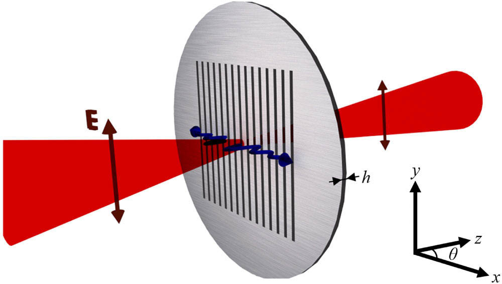
    Fig. 1. Schematic of the metallic subwavelength slit array with dielectric backing of thickness h, illuminated by the focused Gaussian beam with polarization parallel to the slits. The excited leaky waves are depicted by the wavy blue arrows propagating away from the illumination spot. Lattice period dx=0.6  mm, slit width s=0.22  mm, and dielectric thickness h=102 and 188 μm. The scatter angle θ is in the xz-plane.
    Normal transmission spectrum in dB for each of the six samples of thickness (a) 102±1 μm and (b) 188±1 μm, using the collimated (estimated beam diameter, 2wx=7.8 mm) measurement setup. The grey dashed lines indicate the emergence of the Wood’s anomalies. Notice that the second Wood’s anomaly emerges at different frequencies for thin and thick samples, in agreement with the method of moments (see Figs. 7, 8, and 13). Spectra simulated using CST Microwave Studio unit cell boundary conditions and Floquet ports have been overlayed as black dashed lines for comparison.
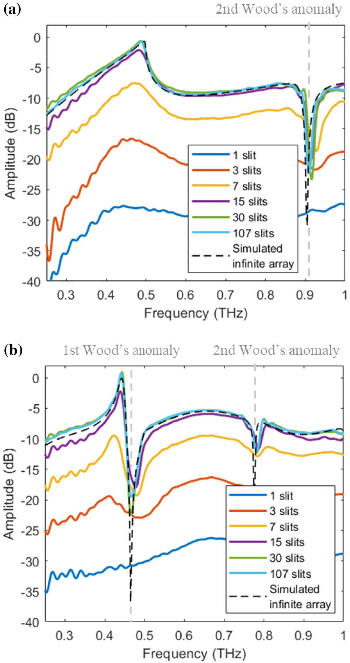
    Fig. 2. Normal transmission spectrum in dB for each of the six samples of thickness (a) 102±1  μm and (b) 188±1  μm, using the collimated (estimated beam diameter, 2wx=7.8  mm) measurement setup. The grey dashed lines indicate the emergence of the Wood’s anomalies. Notice that the second Wood’s anomaly emerges at different frequencies for thin and thick samples, in agreement with the method of moments (see Figs. 7, 8, and 13). Spectra simulated using CST Microwave Studio unit cell boundary conditions and Floquet ports have been overlayed as black dashed lines for comparison.
    Transmission amplitude as a function of the number of slits normalized by the beam diameter for the three different setup configurations, for sample thicknesses of (top) 102±1 μm and (bottom) 188±1 μm, at frequencies 0.48 THz and 0.44 THz, respectively.
    Fig. 3. Transmission amplitude as a function of the number of slits normalized by the beam diameter for the three different setup configurations, for sample thicknesses of (top) 102±1  μm and (bottom) 188±1  μm, at frequencies 0.48 THz and 0.44 THz, respectively.
    Simulated absolute value of the electric field along the structures, calculated in the transient solver of CST Microwave Studio, (a) for sample thickness of 102±1 μm for 7 slits, at ET frequency 0.48 THz and (b), (c) for sample thickness of 188±1 μm for 7 and 107 slits, respectively, at ET frequency 0.44 THz. One half of the array is presented. The end of the seven-slit array is indicated by the white dashed line.
    Fig. 4. Simulated absolute value of the electric field along the structures, calculated in the transient solver of CST Microwave Studio, (a) for sample thickness of 102±1  μm for 7 slits, at ET frequency 0.48 THz and (b), (c) for sample thickness of 188±1  μm for 7 and 107 slits, respectively, at ET frequency 0.44 THz. One half of the array is presented. The end of the seven-slit array is indicated by the white dashed line.
    Spectrograms of the detected waveforms for samples with (a) 7 and (b) 107 slits of thickness 102±1 μm and sample with (c) 107 slits of thickness 188±1 μm. Measurements were taken for the collimated configuration.
    Fig. 5. Spectrograms of the detected waveforms for samples with (a) 7 and (b) 107 slits of thickness 102±1  μm and sample with (c) 107 slits of thickness 188±1  μm. Measurements were taken for the collimated configuration.
    Radiation diagrams for each of the five samples of thickness 102±1 μm (top) and 188±1 μm (bottom), at frequencies 0.48 THz and 0.44 THz, respectively, using the collimated measurement setup.
    Fig. 6. Radiation diagrams for each of the five samples of thickness 102±1  μm (top) and 188±1  μm (bottom), at frequencies 0.48 THz and 0.44 THz, respectively, using the collimated measurement setup.
    Color maps presenting the transmission amplitude in dB as a function of frequency and angle of detection for the three setup configurations, for samples with 107 slits of thicknesses (a) 102±1 μm and (b) 188±1 μm. The scale is the same for all maps, as indicated by the scale bar, to allow for direct comparison. The focused 50 mm lens setup results include an overlaid calculated emission for the diffraction or grating lobe, indicated by the black dashed line, while the space harmonics calculated using method of moments are indicated by the white dashed lines in the same plots, and labeled according to their respective orders. The first and second Wood’s anomalies are indicated by the arrows in the focused 100 mm lens setup results in (b).
    Fig. 7. Color maps presenting the transmission amplitude in dB as a function of frequency and angle of detection for the three setup configurations, for samples with 107 slits of thicknesses (a) 102±1  μm and (b) 188±1  μm. The scale is the same for all maps, as indicated by the scale bar, to allow for direct comparison. The focused 50 mm lens setup results include an overlaid calculated emission for the diffraction or grating lobe, indicated by the black dashed line, while the space harmonics calculated using method of moments are indicated by the white dashed lines in the same plots, and labeled according to their respective orders. The first and second Wood’s anomalies are indicated by the arrows in the focused 100 mm lens setup results in (b).
    Dispersion diagrams calculated from the method of moments for dielectric thicknesses 102 μm (top) and 188 μm (bottom). The real part of the wavevector is presented on the abscissa axis, while the imaginary part is indicated by the color bar on the right. The wavevectors are normalized to the free space wavevector. The orders of the modes are labeled.
    Fig. 8. Dispersion diagrams calculated from the method of moments for dielectric thicknesses 102 μm (top) and 188 μm (bottom). The real part of the wavevector is presented on the abscissa axis, while the imaginary part is indicated by the color bar on the right. The wavevectors are normalized to the free space wavevector. The orders of the modes are labeled.
    Colour map illustrating the dependence of transmission on the slit width s, for samples with dx=0.6 mm and dielectric thicknesses (a) 102 μm and (b) 188 μm, simulated using CST Microwave Studio unit cell boundary conditions and Floquet ports. Note the different scales.
    Fig. 9. Colour map illustrating the dependence of transmission on the slit width s, for samples with dx=0.6  mm and dielectric thicknesses (a) 102 μm and (b) 188 μm, simulated using CST Microwave Studio unit cell boundary conditions and Floquet ports. Note the different scales.
    Decay of electric field along one half of the 188 μm dielectric thick array for varying slit width s, simulated in CST Microwave Studio. The field has been normalized to the maximum field for each measurement. The dashed line illustrates the end of the periodic region of the structure.
    Fig. 10. Decay of electric field along one half of the 188 μm dielectric thick array for varying slit width s, simulated in CST Microwave Studio. The field has been normalized to the maximum field for each measurement. The dashed line illustrates the end of the periodic region of the structure.
    Spectra for varying periodicity dx, for samples with s=0.22 mm and dielectric thicknesses (a) 102 μm and (b) 188 μm, simulated using CST Microwave Studio unit cell boundary conditions and Floquet ports. Note the different scales.
    Fig. 11. Spectra for varying periodicity dx, for samples with s=0.22  mm and dielectric thicknesses (a) 102 μm and (b) 188 μm, simulated using CST Microwave Studio unit cell boundary conditions and Floquet ports. Note the different scales.
    Schematic diagram of the (a) collimated and (b) focused configurations of the TDS setup. The open grey boxes illustrate the photoconductive antenna casings.
    Fig. 12. Schematic diagram of the (a) collimated and (b) focused configurations of the TDS setup. The open grey boxes illustrate the photoconductive antenna casings.
    Dispersion diagrams calculated from the method of moments for h=102 μm (top) and h=188 μm (bottom). The color represents the value of the determinant of the method of moments system in logarithm scale and the dashed lines indicate the modes, which are labeled according to their respective orders.
    Fig. 13. Dispersion diagrams calculated from the method of moments for h=102  μm (top) and h=188  μm (bottom). The color represents the value of the determinant of the method of moments system in logarithm scale and the dashed lines indicate the modes, which are labeled according to their respective orders.
    Simulation of transmission through infinite periodic arrays with h=102 μm (top) and h=188 μm (bottom) using CST Microwave Studio unit cell boundary conditions and Floquet ports. The space harmonics calculated using method of moments are indicated by the white dashed lines. The inset presents a sketch of the simulation demonstrating the off-axis illumination and detection scheme. The blue and grey regions indicate the dielectric material and metal, respectively, while the red arrows indicate the direction of incident and transmitted radiation.
    Fig. 14. Simulation of transmission through infinite periodic arrays with h=102  μm (top) and h=188  μm (bottom) using CST Microwave Studio unit cell boundary conditions and Floquet ports. The space harmonics calculated using method of moments are indicated by the white dashed lines. The inset presents a sketch of the simulation demonstrating the off-axis illumination and detection scheme. The blue and grey regions indicate the dielectric material and metal, respectively, while the red arrows indicate the direction of incident and transmitted radiation.
    Suzanna Freer, Miguel Camacho, Sergei A. Kuznetsov, Rafael R. Boix, Miguel Beruete, Miguel Navarro-Cía. Revealing the underlying mechanisms behind TE extraordinary THz transmission[J]. Photonics Research, 2020, 8(4): 430
    Download Citation