Revealing the underlying mechanisms behind TE extraordinary THz transmission

Suzanna Freer; Miguel Camacho; Sergei A. Kuznetsov; Rafael R. Boix; Miguel Beruete; Miguel Navarro-Cía

doi:10.1364/PRJ.8.000430

Journals >Photonics Research >Volume 8 >Issue 4 >Page 430 > Article

Photonics Research
Vol. 8, Issue 4, 430 (2020)

Revealing the underlying mechanisms behind TE extraordinary THz transmission

Suzanna Freer¹, Miguel Camacho², Sergei A. Kuznetsov^3、4, Rafael R. Boix⁵, Miguel Beruete^6、7, and Miguel Navarro-Cía^1、*

Author Affiliations

¹School of Physics and Astronomy, University of Birmingham, Birmingham B15 2TT, UK

²Department of Physics and Astronomy, University of Exeter, Exeter EX4 4QD, UK

³Rzhanov Institute of Semiconductor Physics SB RAS Novosibirsk Branch TDIAM, Novosibirsk 630090, Russia

⁴Physics Department, Novosibirsk State University, Novosibirsk 630090, Russia

⁵Department of Electronics and Electromagnetism, Faculty of Physics, University of Seville, 41012 Seville, Spain

⁶Antennas Group-TERALAB, Universidad Pública de Navarra, 31006 Pamplona, Spain

⁷Institute of Smart Cities, Universidad Pública de Navarra, 31006 Pamplona, Spain

show less

DOI: 10.1364/PRJ.8.000430 Cite this Article Set citation alerts

Suzanna Freer, Miguel Camacho, Sergei A. Kuznetsov, Rafael R. Boix, Miguel Beruete, Miguel Navarro-Cía. Revealing the underlying mechanisms behind TE extraordinary THz transmission[J]. Photonics Research, 2020, 8(4): 430 Copy Citation Text

EndNote(RIS)

BibTex

Plain Text

show less

Abstract

Transmission through seemingly opaque surfaces, so-called extraordinary transmission, provides an exciting platform for strong light–matter interaction, spectroscopy, optical trapping, and color filtering. Much of the effort has been devoted to understanding and exploiting TM extraordinary transmission, while TE anomalous extraordinary transmission has been largely omitted in the literature. This is regrettable from a practical point of view since the stronger dependence of the TE anomalous extraordinary transmission on the array’s substrate provides additional design parameters for exploitation. To provide high-performance and cost-effective applications based on TE anomalous extraordinary transmission, a complete physical insight about the underlying mechanisms of the phenomenon must be first laid down. To this end, resorting to a combined methodology including quasi-optical terahertz (THz) time-domain measurements, full-wave simulations, and method of moments analysis, subwavelength slit arrays under s-polarized illumination are studied here, filling the void in the current literature. We believe this work unequivocally reveals the leaky-wave role of the grounded-dielectric slab mode mediating in TE anomalous extraordinary transmission and provides the necessary framework to design practical high-performance THz components and systems.

1. INTRODUCTION

Diffraction gratings have been ubiquitous in science and technology for more than a century [1], but scientists still find new physics in them. One of the most remarkable discoveries in this field in the last few decades has been extraordinary optical transmission [2,3]. In the optics community, it became widely accepted that extraordinary transmission (ET) was linked to p-polarized (transverse magnetic, TM) plasmon modes [4]. Subsequent measurements in microwaves [5,6] and terahertz (THz) frequencies [7,8], and theoretical works under perfect electric conductor formalism [9] reinforced the relevance of leaky-type TM modes [10]. However, a few theoretical works largely unnoticed by the community [11–13] also indicated the existence of ET for s-polarized (transverse electric, TE) modes, which was accidentally measured soon thereafter [14] and explicitly reported for different configurations a few years afterward [15–17]. These TE modes are classical grounded-dielectric slab modes [18] that can exist in any region of the spectrum, unlike surface plasmon polaritons.

The activity in TE ET has recently taken off [19–23], driven mainly by applications in quasi-optics [24,25] and sensing [26]. Unlocking the full potential of TE ET would be possible if the same level of understanding as with TM ET is gained in terms of physics and practical considerations. To this end, the work will be positioned within the leaky-wave formalism that provides physical insight as well as design guidelines for high-performance devices, as demonstrated in bull’s eye antennas [10,27] and quasi-optical filters [28].

The array under study here will be an aluminum (Al) truncated subwavelength slit array with lattice period $d_{x} = 0.6 mm$ , slit width $s = 0.22 mm$ , and slit length of 70 mm (see Fig. 1). Such lattice period and slit width are chosen for the ET to emerge in the frequency range where the measurement instrument has its signal peak. The slit length has no effect on the TE ET provided it is significantly longer than the incident beam diameter $2 w_{y}$ . The influence of the slit width and periodicity on the TE ET can be found in Appendix A. We will consider $n = 1$ , 3, 7, 15, 30, and 107 slit samples patterned on polypropylene (PP) ( $ϵ_{r} = 2.25$ [15,28,29]) with varying thicknesses (102 and 188 μm) to characterize frustrated and fully developed TE ET (i.e., when the ${TE}_{1}$ grounded-dielectric slab mode is below or above cutoff [17,19]). Fabrication details can be found elsewhere [29]. The fabricated samples, which will be measured with the TERA K15 all fiber-coupled THz time-domain spectrometer from Menlo Systems under three different experimental conditions as described in Appendix B and in Ref. [30], will be referred to as collimated, 100-focused, and 50-focused. To support the experimental findings and provide further physical insight, full-wave simulations as well as method of moments analysis (which we successfully used for TM ET through subwavelength hole arrays [30]) will be shown (see Appendix B for technical details).

Sign up for Photonics Research TOC. Get the latest issue of Photonics Research delivered right to you！Sign up now

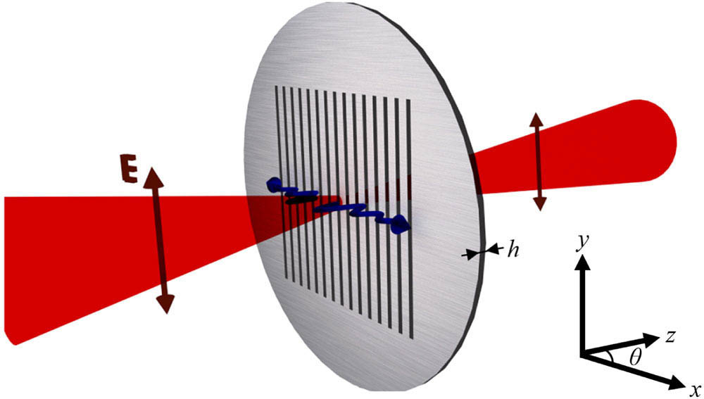
Figure 1.Schematic of the metallic subwavelength slit array with dielectric backing of thickness $h$ , illuminated by the focused Gaussian beam with polarization parallel to the slits. The excited leaky waves are depicted by the wavy blue arrows propagating away from the illumination spot. Lattice period $d_{x} = 0.6 mm$ , slit width $s = 0.22 mm$ , and dielectric thickness $h = 102$ and 188 μm. The scatter angle $θ$ is in the $x z$ -plane.

2. RESULTS AND DISCUSSION

A. Normal Transmission Spectra and ET Saturation

The signature of leaky waves in ET is revealed when transmission is monitored as a function of the number of periods [8,28,30–34] for TM ET in subwavelength hole arrays and [27,35–37] for TM ET inspired highly directive antennas. In order to demonstrate experimentally the influence of the number of slits on the TE ET (frustrated and fully developed), time-domain measurements are taken for the collimated experimental setup, as described in Appendix B. Figure 2 presents the amplitude of normal transmission (i.e., emitter and detector aligned with the axis between them perpendicular to the sample) as a function of frequency, obtained from the Fourier transformation of the waveforms. By comparing Figs. 2(a) and 2(b), one can grasp the critical role that the dielectric substrate thickness plays in the TE ET. When the dielectric substrate is thin (frustrated TE ET), the fundamental grounded-dielectric slab TE mode, ${TE}_{1}$ , is in cutoff (i.e., evanescent) and the minimum associated with the first Rayleigh–Wood’s anomaly ( $\sim 0.47 THz$ ) is suppressed [11,12,17,19,21]. When the dielectric is thick enough (fully developed TE ET), grounded-dielectric slab space harmonics are supported due to the periodicity. They yield an increase in ET compared to the frustrated ET. Additionally, the spectra of these 188 μm thick substrate samples present the characteristic dip linked to the first Wood’s anomaly, known within the leaky-wave formalism as the open stopband [38].

Figure 2.Normal transmission spectrum in dB for each of the six samples of thickness (a) $102 \pm 1 μm$ and (b) $188 \pm 1 μm$ , using the collimated (estimated beam diameter, $2 w_{x} = 7.8 mm$ ) measurement setup. The grey dashed lines indicate the emergence of the Wood’s anomalies. Notice that the second Wood’s anomaly emerges at different frequencies for thin and thick samples, in agreement with the method of moments (see Figs. 7, 8, and 13). Spectra simulated using CST Microwave Studio unit cell boundary conditions and Floquet ports have been overlayed as black dashed lines for comparison.

For the cases where the patterned area is smaller than the incident Gaussian beam (i.e., between 1 and 15 slits), transmission increases with the number of slits throughout the whole spectral window due to the growing clear area. This direct transmission saturates when the patterned area is as large as the incident Gaussian beam. However, the maximum transmission does not saturate at this point (also see blue line in Fig. 3). An additional enhancement at the ET frequency is evident at $\sim 0.4 - 0.5 THz$ , starting from three slits, especially for 188 μm thick substrate samples. This extra increase can be attributed to the $m = - 1$ space harmonic of the ${TE}_{1}$ grounded-dielectric slab mode, as demonstrated conclusively later. Notice that for a large numbers of slits, the fully developed TE ET is above 0 dB. This is due to collimation at broadside, resulting from the contribution of the leaky-wave associated with the $m = - 1$ space harmonic of the ${TE}_{1}$ grounded-dielectric slab mode, and it does not violate the law of conservation of energy; the slit array simply redirects the energy more effectively toward the detection area than the measurement without the sample (i.e., calibration). This saturation effect [28,30] and transmission above 0 dB have been reported for TM ET through subwavelength hole arrays [30], but not yet for TE ET.

Figure 3.Transmission amplitude as a function of the number of slits normalized by the beam diameter for the three different setup configurations, for sample thicknesses of (top) $102 \pm 1 μm$ and (bottom) $188 \pm 1 μm$ , at frequencies 0.48 THz and 0.44 THz, respectively.

To highlight the leaky-wave mechanism, it is convenient to monitor the ET amplitude as a function of the array size (i.e., the number of slits multiplied by the periodicity, $d_{x}$ ) to illumination-spot-size ( $2 w_{x}$ ) ratio [28], since the leaky-wave contribution depends inherently on the number of periods, but is independent of the illumination beam spot. To this end, both substrate-thin and substrate-thick samples are illuminated with estimated beam diameters of $\sim 7.8 mm$ , $\sim 5.9 mm$ , and $\sim 3.0 mm$ for the collimated, focused with 100 mm lens and focused with 50 mm lens configurations, respectively (see Fig. 3). The results reveal the fundamental distinction between the number of directly illuminated slits and the total number of slits participating in the resonance process. Saturated transmission is only achieved when the array length is larger ( $\sim 30$ slits, corresponding to $n d_{x} / 2 w_{x}$ of $\sim 6$ , for the 50-focused setup) than the beam diameter. Figure 3 also demonstrates that transmission through the thicker sample reaches a higher saturation amplitude consistently for all three configurations, indicating the need for the ${TE}_{1}$ mode to be propagating for a more efficient ET.

The dependency of sufficient number of slits and dielectric thickness is supported through calculation of the absolute value of the electric field on the $x z$ -plane, simulated in the transient solver of CST Microwave Studio with Gaussian beam illumination. Figure 4 presents the field for a substrate-thin sample with 7 slits, and two substrate-thick samples, with 7 and 107 slits. The presence of an electric field within the dielectric slab beyond the illumination area in Fig. 4(c) with respect to Fig. 4(a), demonstrates the development of the $m = - 1$ mode, as the substrate thickness is increased above a threshold. For the thick-dielectric sample, a more efficient coupling of energy to the $m = - 1$ leaky mode can be observed in the structure with 107 slits [Fig. 4(c)] in comparison to seven slits [Fig. 4(b)], supporting the results in Fig. 3. The increase in the number of slits means the incident energy couples to the leaky $m = - 1$ space harmonic of the ${TE}_{1}$ mode, rather than the slow, confined ${TE}_{1}$ wave, which is observed travelling along the nonperiodic region of the seven-slit structure in Fig. 4(b). The energy coupled to this slow mode remains in the structure, without radiating to free space, unlike the leaky mode, which reradiates energy, increasing ET.

Figure 4.Simulated absolute value of the electric field along the structures, calculated in the transient solver of CST Microwave Studio, (a) for sample thickness of $102 \pm 1 μm$ for 7 slits, at ET frequency 0.48 THz and (b), (c) for sample thickness of $188 \pm 1 μm$ for 7 and 107 slits, respectively, at ET frequency 0.44 THz. One half of the array is presented. The end of the seven-slit array is indicated by the white dashed line.

The characteristic of the leaky $m = - 1$ space harmonic of the ${TE}_{1}$ mode, and thus, of the ET saturation condition can be modulated via the slit width. Full-wave simulations of the lossless case (i.e., using perfect electric conductor and a lossless PP) show how the leakage constant increases with the slit width (see Appendix A).

B. Temporal Dependence of Transmission

The coupling between the incident Gaussian beam and the $m = - 1$ space harmonic (of the ${TE}_{1}$ grounded-dielectric slab mode) mediating in the ET is resonant in nature [11,12]. In addition, because of the leaky-wave nature of the $m = - 1$ space harmonic, time-delayed energy contribution akin to that observed in bull’s eye antennas [39] should be detected in the time-resolved measurements. To observe such energy retention within the system, we now carry out a temporal analysis not reported before for TE ET. Figure 5 presents spectrograms (i.e., time-frequency maps) for two 102 μm samples with seven and 107 slits and one 188 μm sample with 107 slits, measured using the collimated setup. The results demonstrate the prolonged presence of energy in the system after illumination, at the frequency of the ET peak. As elucidated above, this is mainly attributed to the longer path (i.e., time delay)—compared to the direct transmission—followed by the energy that couples to the leaky wave that propagates along the array before being re-emitted toward the detector. For a larger number of slits, the leaky waves can propagate for longer. Hence, longer ringing is observed for 107 slits compared to seven slits [Figs. 5(a) and 5(b)]. The fact that the ${TE}_{1}$ mode is in cutoff for substrate-thin samples constrains ringing to $\sim 20 ps$ . For the substrate-thick sample, the ${TE}_{1}$ mode is above cutoff and its $m = - 1$ leaky wave can explore a large number of slits, resulting in a significantly longer ringing of energy ( $\sim 45 ps$ ), as shown in Fig. 5(c).

Figure 5.Spectrograms of the detected waveforms for samples with (a) 7 and (b) 107 slits of thickness $102 \pm 1 μm$ and sample with (c) 107 slits of thickness $188 \pm 1 μm$ . Measurements were taken for the collimated configuration.

C. Angle-Resolved Transmission

Normal transmission measurements provide some physical insight into the TE ET. Nevertheless, complete understanding of the underlying mechanisms in TE ET requires the study of the sample’s angular emission and the correlation of the measurements with numerical simulations to isolate the physics from instrument-induced artifacts [30]. Indeed, the presence of leaky waves should have a strong effect on the radiating properties of the array [27,28,30,33,36–38] for TM ET and [16,35] for TE ET in a slit flanked by corrugations. Hence, the angle-resolved transmission amplitude on the H-plane ( $x z$ -plane, as indicated in Fig. 1) at the ET peak frequency for each sample is presented in Fig. 6. As the number of slits increases, the beamwidth of the main lobe narrows down (notice that it saturates around the same number of slits as in Fig. 3) while emission beyond 10 deg is drastically reduced. For large angles of emission, interference fringes are visible. This signature stems from the interference of the different illuminated slits. Hence, the number of nodes and antinodes increases with the number of slits.

Figure 6.Radiation diagrams for each of the five samples of thickness $102 \pm 1 μm$ (top) and $188 \pm 1 μm$ (bottom), at frequencies 0.48 THz and 0.44 THz, respectively, using the collimated measurement setup.

For the substrate-thin samples [Fig. 6(a)], the maximum appears at 0 deg (i.e., broadside). However, for the substrate-thick samples with large number of slits [Fig. 6(b)], the maximum emerges at 1 deg. This finding is consistent with the leaky-wave formalism. In substrate-thick samples with a large number of slits, the leaky wave associated with the ${TE}_{1}$ grounded-dielectric slab mode plays a major role in the ET. Because of the open stopband, however, the contribution of the $m = - 1$ space harmonic (of the ${TE}_{1}$ grounded-dielectric slab mode) must vanish at broadside [38].

To shed more light on the angular dependence and leaky-wave mechanism of subwavelength hole arrays in addition to the influence of the quasi-optics in the measurement, Figs. 7(a) and 7(b) present angle-resolved transmission spectra as radiation diagrams for thin- and thick-dielectric samples, respectively, for each of the three setups: collimated, 100-focused, and 50-focused.

$Color maps presenting the transmission amplitude in dB as a function of frequency and angle of detection for the three setup configurations, for samples with 107 slits of thicknesses (a) 102±1 μm and (b) 188±1 μm. The scale is the same for all maps, as indicated by the scale bar, to allow for direct comparison. The focused 50 mm lens setup results include an overlaid calculated emission for the diffraction or grating lobe, indicated by the black dashed line, while the space harmonics calculated using method of moments are indicated by the white dashed lines in the same plots, and labeled according to their respective orders. The first and second Wood’s anomalies are indicated by the arrows in the focused 100 mm lens setup results in (b).$

Figure 7.Color maps presenting the transmission amplitude in dB as a function of frequency and angle of detection for the three setup configurations, for samples with 107 slits of thicknesses (a) $102 \pm 1 μm$ and (b) $188 \pm 1 μm$ . The scale is the same for all maps, as indicated by the scale bar, to allow for direct comparison. The focused 50 mm lens setup results include an overlaid calculated emission for the diffraction or grating lobe, indicated by the black dashed line, while the space harmonics calculated using method of moments are indicated by the white dashed lines in the same plots, and labeled according to their respective orders. The first and second Wood’s anomalies are indicated by the arrows in the focused 100 mm lens setup results in (b).

The ET peak occurs for a frequency range 0.4–0.5 THz for small angles, consistent with the $m = - 1$ leaky mode. Additional space harmonics are evident in the focused 50 mm lens setup, while their angular dependencies are consistent with method of moments (see technical details in Appendix B) calculations, presented as dispersion diagrams in Fig. 8. At large angles of detection, transmission resulting from the diffraction lobe of scattered fields of the incident beam (i.e., space harmonic $m = - 1$ related to the incident field and the periodicity, but not to the grounded-dielectric slab mode) is detected, indicated by the black dashed line. The far field transmission for an infinite array was also simulated using the commercial software CST Microwave Studio and the results obtained (not shown) are in agreement with Fig. 7.

Figure 8.Dispersion diagrams calculated from the method of moments for dielectric thicknesses 102 μm (top) and 188 μm (bottom). The real part of the wavevector is presented on the abscissa axis, while the imaginary part is indicated by the color bar on the right. The wavevectors are normalized to the free space wavevector. The orders of the modes are labeled.

The two high-transmission branches stemming from 0.46 THz at 0 deg are the $m = - 1$ leaky mode. They exhibit a higher angular dependence for the configuration with the 50 mm lens since the focused field is incident on the sample at larger angles to the surface normal, and the collection lens increases the numerical aperture of the detector. This behavior is consistent with the simulation results, which are presented as a surface plot in Appendix D. An additional narrow resonance emerged between the aforementioned bands with negligible angular dispersion. This is thought to be a result of the $m = - 1$ asymmetric mode [15,40], known as the odd mode in the circuit model formalism, which only appears in relative thick screens with very low ohmic losses [41].

For thin-dielectric samples, the $m = - 1$ mode is a pseudomode up to $\sim 0.66 THz$ since the ${TE}_{1}$ grounded-dielectric slab mode is in cutoff below such a frequency. Hence, the determinant of the method of moments does not have a zero, but a minimum instead, up to $\sim 0.66 THz$ (see Appendix C). It is also worth noticing that such $m = - 1$ pseudomode vanishes for $k_{x_{0}} \to 0$ [see Figs. 7(a) and Appendix D]. As a result, the ET peak is always below 0 dB under normal incidence illumination (see Fig. 2). For thick-dielectric samples, the cutoff frequency for a ${TE}_{1}$ grounded-dielectric slab mode is $\sim 0.36 THz$ . The corresponding $m = - 1$ space harmonic does not vanish as $k_{x_{0}} \to 0$ and crosses the $k_{x_{0}} = 0$ axis with a large $Im (k_{x_{0}})$ below the Rayleigh–Wood’s anomaly [Fig. 8(b)], which is the signature of ET.

3. CONCLUSION

In short, we believe this paper has shed more light on the largely unnoticed TE extraordinary transmission, both in the fully developed and frustrated versions. We believe we have unequivocally revealed the leaky-wave role governing the fully developed TE extraordinary transmission—like TM extraordinary transmission. The leaky-wave mechanism has two main implications from a practical point of view. On the one hand, a larger number of slits than those directly illuminated are needed to achieve saturation of transmission above 0 dB; the frustrated TE extraordinary transmission also saturates with the number of slits, but does not reach 0 dB since the associated mode vanishes for normal incidence below the first Rayleigh–Wood’s anomaly. On the other hand, quasi-optical setups with different angular distributions upon illumination and collection (i.e., using different numerical aperture lenses/mirrors) provide different angle-frequency transmission maps because of the different excitations of the variety of leaky modes sustained by the subwavelength slit array. The measurements reported here highlight the challenges regarding the calibration of quasi-optical THz systems for structures that have underlying leaky-wave mechanisms.

Acknowledgment

Acknowledgment. The authors would like to thank Dr. V. Pacheco-Peña for his advice regarding Fig. 1, and Ms. E. Shalom and Mr. J. Gape for the beam radius estimations.

APPENDIX A: SLIT DIMENSION INFLUENCE ON TE ET

CST Microwave Studio was used to simulate the array with varying slit width $s$ and periodicity $d_{x}$ . (See technical details of the simulations in Appendix B.) Here, ohmic and dielectric losses have been neglected to remove their contributions to the decay of the leaky waves.

Figure 9 illustrates the spectral dependence on the slit width, while Fig. 10 presents the decay of a normalized electric field along the $x$ -axis, as shown in Fig. 1. Figure 10 demonstrates that the larger the slit width, the larger the leakage per period is, resulting in the leaky wave propagating for a shorter period before completely decaying. These results are consistent with $| Im (k_{x 0}) | / k_{0}$ calculated with the method of moments at the corresponding ET frequency: $| Im [k_{x 0} (s = 0.18)] | / k_{0} = 236$ , $| Im [k_{x 0} (s = 0.22)] | / k_{0} = 307$ , and $| Im [k_{x 0} (s = 0.26)] | / k_{0} = 333$ .

Figure 11 presents the simulated spectra for varying periodicity $d_{x}$ . There is an observable shift of the ET peak toward lower frequencies with increasing periodicity for samples with both dielectric thicknesses.

Figure 9.Colour map illustrating the dependence of transmission on the slit width $s$ , for samples with $d_{x} = 0.6 mm$ and dielectric thicknesses (a) 102 μm and (b) 188 μm, simulated using CST Microwave Studio unit cell boundary conditions and Floquet ports. Note the different scales.

Figure 10.Decay of electric field along one half of the 188 μm dielectric thick array for varying slit width $s$ , simulated in CST Microwave Studio. The field has been normalized to the maximum field for each measurement. The dashed line illustrates the end of the periodic region of the structure.

Figure 11.Spectra for varying periodicity $d_{x}$ , for samples with $s = 0.22 mm$ and dielectric thicknesses (a) 102 μm and (b) 188 μm, simulated using CST Microwave Studio unit cell boundary conditions and Floquet ports. Note the different scales.

APPENDIX B: METHODS

Experimental Setup: The samples were characterized using an all fiber-coupled THz time-domain spectrometer TERA K15 with lock-in detection (Menlo Systems). The time-constant was set to 300 ms. The temporal length of the waveforms was 261 ps, providing a spectral resolution of 4.8 GHz.

The detector was installed on a rotating mount to allow for measurements in a range of angles with respect to the source-sample axis (i.e., scatterometer) [30]. The distance between the detector and sample was approximately 110 mm. Three different optical configurations were used to characterize the samples. Setup 1 used collimated illumination, providing an estimated frequency dependent beam diameter along the $x$ -axis (indicated in Fig. 12) of 7.8 mm at 0.5 THz at the sample position (see Fig. 12). Setups 2 and 3 used focused illumination through the installation of a lens before the sample. TPX100 and TPX50 planoconvex lenses, of effective focal lengths 100 mm and 50 mm, were used to provide estimated beam diameters along the $x$ -axis of 5.9 and 3.0 mm at the sample position, for setups 2 and 3, respectively. It should be noted that a truly collimated field cannot be achieved with photoconductive antennas. Hence, the incident field is slightly diverging in these measurements.

Figure 12.Schematic diagram of the (a) collimated and (b) focused configurations of the TDS setup. The open grey boxes illustrate the photoconductive antenna casings.

The photoconductive antennas used in the spectrometer produced a vertically linearly polarized field, aligned along the slit direction. The different lenses of the quasi-optical system may induce some degradation of the polarization purity that was not considered in the measurements or numerical analysis. To enhance the polarization purity at the sample position, it would be advisable to position a linear polarizer along the beam path.

Scans were recorded at varying angles on the H-plane ( $x z$ -plane) in increments of 1 deg up to 20 deg, 2.5 deg between 20 deg and 40 deg (50 deg for setup 2), and then 5 deg up to 55 deg.

Data Processing: Prior to performing a Fourier transform on the time-domain data, the data was subject to time-windowing using a Hanning-type window. Measurements were calibrated through comparison to a measurement taken without the sample with the source and detector on-axis, on the day of the experiment. The calibration data was removed from the signal data in the frequency domain. The results in Fig. 2 were filtered using a lowpass filter, with a cutoff frequency 0.2 THz, while the spectrograms in Fig. 5 were obtained using an overlap of 98% of the zero-padding length and a number of DFT points of 512.

Simulations: The transient and frequency solvers of CST Microwave Studio were used to simulate the response of the semi-infinite and infinite array under a normal incidence two-dimensional (2D) Gaussian beam, and a normal as well as oblique incidence (i.e., the subwavelength slit array is rotated along $y$ -axis) plane wave excitation, respectively. For the Gaussian beam setup, top and bottom electric walls were defined while the solver-defined open add space boundary conditions were set in $x$ . For the plane wave excitation, the solver-defined unit cell and periodic boundary conditions were employed to generate Figs. 9, 11, and 14, and results related to Fig. 7 that are not shown, respectively. Metal was modeled with conductivity $σ = 3.56 \times 10^{7} S / m$ , except for Appendix A (Figs. 9–11) where the perfect electric conductor is considered. The PP was modeled as $_{r} = 2.25$ and loss tangent $\tan δ = 10^{3}$ , except for Appendix A, where it was considered as a perfect lossless dielectric.

Method of moments: This numerical technique is employed for the solution of the integral equation satisfied by the electric field on the surface of the slits in zero-thickness perfect electric conductor (PEC) plates supported by a grounded dielectric slab. Because we are interested in the self-supported surface waves, no excitation is considered and the integral equation is given by $\int_{\frac{s}{2}}^{\frac{s}{2}} \int_{\infty}^{\infty} {\overset{ˉ}{G}}^{per} (x x^{'}, y y^{'}) \cdot E_{t} (x^{'}, y^{'}) d x^{'} d y^{'} = 0$ (B1)for $\frac{s}{2} < x < \frac{s}{2}$ and $\infty < y < \infty$ , where $E_{t} (x, y)$ stands for the unknown tangential electric field distribution on the surface of the $m$ th slit and the kernel of the integral equation corresponds to the 1D periodic dyadic Green’s function relating the electric current and the tangential electric field on the surface of the screen. This periodic Green’s function can be related to the nonperiodic Green’s function through Bloch’s theorem as ${\overset{ˉ}{G}}^{per} (x, y) = \sum_{m = \infty}^{\infty} \overset{ˉ}{G} (x m d_{x}, y) e^{j k_{x 0} m d_{x}},$ (B2)where the phasing $k_{x_{0}} d_{x}$ is imposed between two adjacent unit cells. Following the work in Ref. [42], this integral equation can be solved in the spectral domain [i.e., using the Fourier transform of Eq. (B1)] by providing a limited set of basis functions that can accurately render the behavior of the electric field distribution in the slot and that have an analytical Fourier transform. By using the same basis functions as weighting functions (Galerkin’s version of method of moments) and integrating the result over the unit cell slit, one achieves a system of linear equations for the coefficients of such basis functions. The eigenmode solutions are then retrieved by looking for the zeroes of the determinant of such a system for each frequency and for each phasing between adjacent unit cells, as explained in Ref. [43].

As shown in Refs. [30,42,43] for slits and slots, a very limited set of basis functions is required to achieve convergence when one resorts to the use of Chebyshev polynomials weighted by the right edge behavior for the polarization of interest. In the case of polarization parallel or perpendicular to the slit, the edge behavior is given by a square root zero or square root singularity, respectively, as one approaches the thin metal edge.

APPENDIX C: DISPERSION DIAGRAMS COMPUTED WITH THE METHOD OF MOMENTS

Figure 13.Dispersion diagrams calculated from the method of moments for $h = 102 μm$ (top) and $h = 188 μm$ (bottom). The color represents the value of the determinant of the method of moments system in logarithm scale and the dashed lines indicate the modes, which are labeled according to their respective orders.

APPENDIX D: TRANSMISSION SPECTRA AS A FUNCTION OF ARRAY ROTATION ALONG THE Y-AXIS

Figure 14.Simulation of transmission through infinite periodic arrays with $h = 102 μm$ (top) and $h = 188 μm$ (bottom) using CST Microwave Studio unit cell boundary conditions and Floquet ports. The space harmonics calculated using method of moments are indicated by the white dashed lines. The inset presents a sketch of the simulation demonstrating the off-axis illumination and detection scheme. The blue and grey regions indicate the dielectric material and metal, respectively, while the red arrows indicate the direction of incident and transmitted radiation.

References

[1] P. F. Goldsmith. Quasioptical Systems: Gaussian Beam Quasioptical Propogation and Applications(1998).

[2] E. Betzig, A. Lewis, A. Harootunian, M. Isaacson, E. Kratschmer. Near field scanning optical microscopy (NSOM): development and biophysical applications. Biophys. J., 49, 269-279(1986).

[3] T. W. Ebbesen, H. J. Lezec, H. F. Ghaemi, T. Thio, P. A. Wolff. Extraordinary optical transmission through sub-wavelength hole arrays. Nature, 391, 667-669(1998).

[4] F. J. Garcia-Vidal, L. Martin-Moreno, T. W. Ebbesen, L. Kuipers. Light passing through subwavelength apertures. Rev. Mod. Phys., 82, 729-787(2010).

[5] A. P. Hibbins, B. R. Evans, J. R. Sambles. Experimental verification of designer surface plasmons. Science, 308, 670-672(2005).

[6] M. Beruete, M. Sorolla, I. Campillo, J. S. Dolado, L. Martín-Moreno, J. Bravo-Abad, F. J. García-Vidal. Enhanced millimeter-wave transmission through subwavelength hole arrays. Opt. Lett., 29, 2500-2502(2004).

[7] F. Miyamaru, T. Kondo, T. Nagashima, M. Hangyo. Large polarization change in two-dimensional metallic photonic crystals in subterahertz region. Appl. Phys. Lett., 82, 2568-2570(2003).

[8] T. Matsui, A. Agrawal, A. Nahata, Z. V. Vardeny. Transmission resonances through aperiodic arrays of subwavelength apertures. Nature, 446, 517-521(2007).

[9] J. B. Pendry, L. Martín-Moreno, F. J. García-Vidal. Mimicking surface plasmons with structured surfaces. Science, 305, 847-848(2004).

[10] D. R. Jackson, A. A. Oliner, T. Zhao, J. T. Williams. Beaming of light at broadside through a subwavelength hole: leaky wave model and open stopband effect. Radio Sci., 40, RS6510(2005).

[11] V. Lomakin, E. Michielssen. Enhanced transmission through metallic plates perforated by arrays of subwavelength holes and sandwiched between dielectric slabs. Phys. Rev. B, 71, 235117(2005).

[12] V. Lomakin, E. Michielssen. Transmission of transient plane waves through perfect electrically conducting plates perforated by periodic arrays of subwavelength holes. IEEE Trans. Antennas Propag., 54, 970-984(2006).

[13] E. Moreno, L. Martín-Moreno, F. J. García-Vidal. Extraordinary optical transmission without plasmons: the s-polarization case. J. Opt. A, 8, S94-S97(2006).

[14] M. Beruete, M. Sorolla, M. Navarro-Cía, F. Falcone, I. Campillo, V. Lomakin. Extraordinary transmission and left-handed propagation in miniaturized stacks of doubly periodic subwavelength hole arrays. Opt. Express, 15, 1107-1114(2007).

[15] S. A. Kuznetsov, M. Navarro-Cía, V. V. Kubarev, A. V. Gelfand, M. Beruete, I. Campillo, M. Sorolla. Regular and anomalous extraordinary optical transmission at the THz-gap. Opt. Express, 17, 730-738(2009).

[16] M. Guillaume, A. Y. Nikitin, M. J. K. Klein, L. A. Dunbar, V. Spassov, R. Eckert, L. Martín-Moreno, F. J. García-Vidal, R. P. Stanley. Observation of enhanced transmission for s-polarized light through a subwavelength slit. Opt. Express, 18, 9722-9727(2010).

[17] M. Beruete, M. Navarro-Cía, S. A. Kuznetsov, M. Sorolla. Circuit approach to the minimal configuration of terahertz anomalous extraordinary transmission. Appl. Phys. Lett., 98, 014106(2011).

[18] A. Ishimaru. Electromagnetic Wave Propagation, Radiation, and Scattering(1991).

[19] M. Beruete, M. Navarro-Cía, M. Sorolla-Ayza. Understanding anomalous extraordinary transmission from equivalent circuit and grounded slab concepts. IEEE Trans. Microw. Theory Tech., 59, 2180-2188(2011).

[20] I. Schwarz, N. Livneh, R. Rapaport. General closed-form condition for enhanced transmission in subwavelength metallic gratings in both TE and TM polarizations. Opt. Express, 20, 426-439(2012).

[21] K. S. Reichel, P. Y. Lu, S. Backus, R. Mendis, D. M. Mittleman. Extraordinary optical transmission inside a waveguide: spatial mode dependence. Opt. Express, 24, 28221-28227(2016).

[22] M. Camacho, R. R. Boix, F. Medina, A. P. Hibbins, J. R. Sambles. On the extraordinary optical transmission in parallel plate waveguides for non-TEM modes. Opt. Express, 25, 24670-24677(2017).

[23] Y. Xie, H. Liu, H. Jia, Y. Zhong. Surface-mode model of the extraordinary optical transmission without plasmons. Opt. Express, 23, 5749-5762(2015).

[24] M. Navarro-Cía, P. Rodríguez-Ulibarri, V. Torres, M. Beruete. Quarter-wave plate based on dielectric-enabled extraordinary resonant transmission. IEEE Photon. Technol. Lett., 24, 945-947(2012).

[25] J. W. He, X. K. Wang, Z. W. Xie, Y. Z. Xue, S. Wang, Y. Zhang. Reconfigurable terahertz grating with enhanced transmission of TE polarized light. APL Photon., 2, 076102(2017).

[26] I. Jáuregui-López, P. Rodríguez-Ulibarri, S. A. Kuznetsov, N. A. Nikolaev, M. Beruete. THz sensing with anomalous extraordinary optical transmission hole arrays. Sensors, 18, 3848(2018).

[27] M. Beruete, U. Beaskoetxea, T. Akalin. Flat corrugated and bull’s-eye antennas. Aperture Antennas for Millimeter and Sub-Millimeter Wave Applications, 111-141(2018).

[28] M. Navarro-Cía, V. Pacheco-Peña, S. A. Kuznetsov, M. Beruete. Extraordinary THz transmission with a small beam spot: the leaky wave mechanism. Adv. Opt. Mater., 6, 1701312(2018).

[29] M. Navarro-Cía, S. A. Kuznetsov, M. Aznabet, F. F. M. Beruete, M. Sorolla-Ayza. Route for bulk millimeter wave and terahertz metamaterial design. IEEE J. Quantum Electron., 47, 375-385(2011).

[30] M. Camacho, R. R. Boix, S. A. Kuznetsov, M. Beruete, M. Navarro-Cía. Far-field and near-field physics of extraordinary THz transmitting hole-array antennas. IEEE Trans. Antennas Propag., 67, 6029-6038(2019).

[31] F. Miyamaru, M. Hangyo. Finite size effect of transmission property for metal hole arrays in subterahertz region. Appl. Phys. Lett., 84, 2742-2744(2004).

[32] M. Beruete, M. Sorolla, I. Campillo, J. S. Dolado. Increase of the transmission in cut-off metallic hole arrays. IEEE Microw. Wireless. Compon. Lett., 15, 116-118(2005).

[33] J. Bravo-Abad, A. Degiron, F. Przybilla, C. Genet, F. J. García-Vidal, L. Martín-Moreno, T. W. Ebbesen. How light emerges from an illuminated array of subwavelength holes. Nat. Phys., 2, 120-123(2006).

[34] M. Camacho, R. R. Boix, F. Medina. Computationally efficient analysis of extraordinary optical transmission through infinite and truncated subwavelength hole arrays. Phys. Rev. E, 93, 063312(2016).

[35] A. Y. Nikitin, F. J. García-Vidal, L. Martín-Moreno. Enhanced optical transmission, beaming and focusing through a subwavelength slit under excitation of dielectric waveguide modes. J. Opt. A, 11, 125702(2009).

[36] U. Beaskoetxea, V. Pacheco-Peña, B. Orazbayev, T. Akalin, S. Maci, M. Navarro-Cía, M. Beruete. 77-GHz high-gain bull’s-eye antenna with sinusoidal profile. IEEE Antennas Wireless Propag. Lett., 14, 205-208(2015).

[37] U. Beaskoetxea, S. Maci, M. Navarro-Cía, M. Beruete. 3D-printed 96 GHz bull’s-eye antenna with off-axis beaming. IEEE Trans. Antennas Propag., 65, 17-25(2017).

[38] D. R. Jackson, A. A. Oliner. Modern Antenna Handbook(2017).

[39] A. Agrawal, H. Cao, A. Nahata. Time-domain analysis of enhanced transmission through a single subwavelength aperture. Opt. Express, 13, 3535-3542(2005).