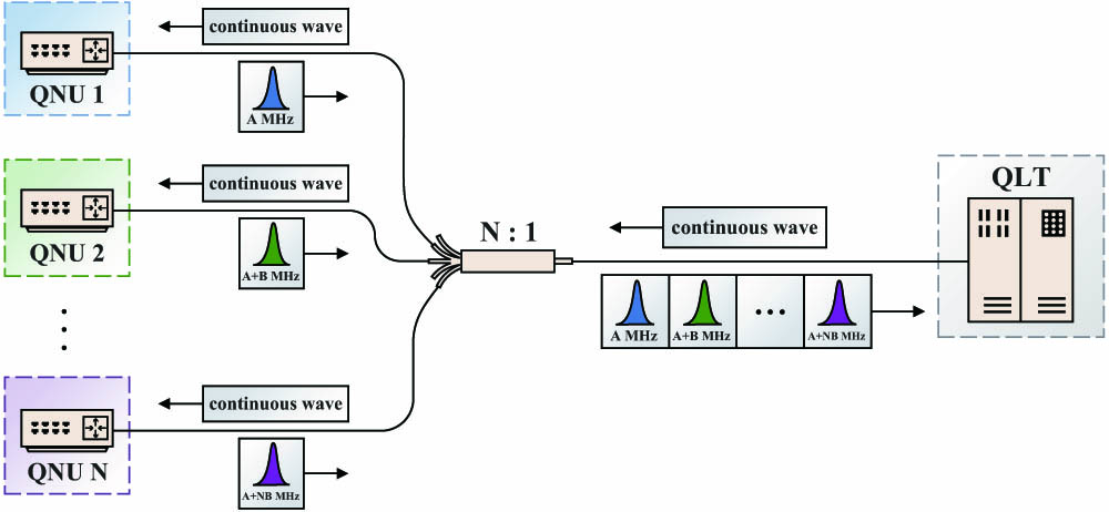
Fig. 1. Schematic diagram of the round-trip multi-band quantum access network (RM-QAN). First, a continuous wave is generated and transmitted by the quantum line terminal (QLT). Then, the continuous wave is divided into N pieces through an N:1 splitter. The quantum network unit (QNU) modulates the key information on different carrier frequencies to be distinguished clearly on the spectrum. Then the key is transmitted back through the round-trip structure, and the modulated signal light is returned to the splitter. Finally, the signal light is passed back to the QLT, which demodulates the received signal.

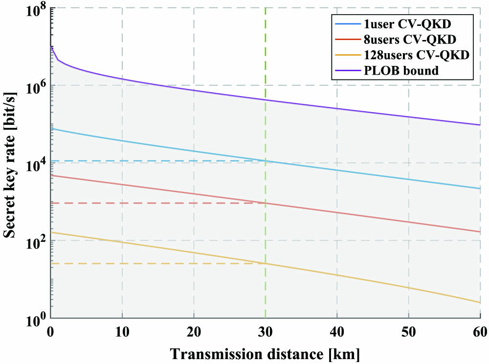
Fig. 2. Comparison diagram of secret key rate between this scheme of different network capacities and other classical schemes. Parameters are set as η=0.42, vel=0.18, β=0.97, VA=0.5  SNU (shot noise unit), R=1  MHz. It describes the change of secret key rate at different transmission distances in the Pirandola–Laurenza–Ottaviani–Banchi (PLOB) bound and round-trip multi-band continuous-variable quantum key distribution (CV-QKD) with different users, where the ordinate value corresponding to the dotted line is the secret key rate under the condition of 30 km achieved in theory.

Fig. 3. Relationship among network capacity, transmission distance, and secret key rate. Parameters are set as η=0.42, vel=0.18, β=0.97, VA=0.5  SNU, R=1  MHz. It describes the change of secret key rate at different transmission distances and different network capacities. The legend on the right shows the value of the secret key rate of each user. (a) Network capacity is eight. (b) Network capacity is 64. (c) Network capacity is 128.

Fig. 4. Optical configuration of the round-trip multi-band scheme. First, the light transmitted by the laser of QLT is divided into two parts by a beam splitter (BS) with a 2:1 ratio. The light of higher power acts as the local oscillator (LO) of the system. The light of lower power passes through a variable optical attenuator (VOA) to the optical circulator. Light is transmitted from port1 to port2 of the optical circulator and to the 30 km optical fiber spool. Afterward, a continuous wave is transmitted to a BS through the optical fiber spool. After arriving at the QNU, light is transmitted to a VOA through port2 to port3 of the optical circulator, and then enters a phase modulator (PM) for signal modulation. Afterward, the signal light enters the polarization controller (PC). After passing through the PC, it enters through port1 of the optical circulator, exits through port2, and returns to BS. After passing through the optical fiber spool again, the signal light enters from port2 of the optical circulator at the QLT and comes out from port3. Then the signal light reaches the PC of QLT. Finally, the signal light and LO light enter the integrated coherent receiver (ICR).

Fig. 5. Spectrum diagram of the signal obtained by QLT through the coherent receiver. It describes the change of amplitude at different frequencies.

Fig. 6. (a) Signal constellation of QNU1, with VA=0.5587  SNU. (b) Signal constellation of QNU2, with VA=0.5170  SNU. (c) Signal constellation of QNU3, with VA=0.5641  SNU. The data in the figure were obtained through several experiments, where k represents different states in discrete modulation coherent state (DMCS) CV-QKD. Different values of k correspond to different colors.

Fig. 7. Cross-correlation of the signal modulated by three QNUs and the signal received by QLT. It describes the change of the cross-correlation of three QNUs at different frames, where the red points represent the successful result.

Fig. 8. Excess noise scatter diagram of three QNUs. It describes the change of the excess noise of three QNUs at different times, where the red line represents the mean value of excess noise of three QNUs. The mean excess noise of QNU1, QNU2, and QNU3 is 0.0054 SNU, 0.0040 SNU, and 0.0059 SNU, respectively.

Fig. 9. Secret key rate curves of the three QNUs in the experiment. It describes the change of the secret key rate of three QNUs at different transmission distances, where the ordinate value corresponding to the dotted line is the secret key rate under the condition of 30 km achieved in our experiment. The secret key rate of QNU1 is 825.82 bit/s, the secret key rate of QNU2 is 674.46 bit/s, and the secret key rate of QNU3 is 635.95 bit/s.

Fig. 10. Relationship between Rayleigh backscattering noise and transmission distance. Parameters are set as β=−40  dB, α=0.2  dB/km, VA=0.5  SNU, R=1  MHz, τ=1  ns, LQNU=3  dB. It describes the change of Rayleigh backscattering noise at different transmission distances.

Fig. 11. Relation between frequency interval and frequency division noise under different modulation variances. Parameters are set as a=27.27, b=−2.066. Hollow points are obtained by the Monte Carlo method, and curves are obtained by nonlinear fitting. It describes the change of frequency division noise at different frequency intervals and different modulation variances (VA).

Fig. 12. Relation between network capacity and frequency cross talk noise. Parameters are set as c=3.815×10−3, d=−0.4576. Hollow points are obtained by the Monte Carlo method, and curves are obtained by nonlinear fitting. The inset shows what happens when the network capacity is large. It describes the change of frequency cross talk noise at different network capacities.

Fig. 13. Schematic diagram of optical circulator noise. The optical circulator of QLT receives light from the laser at port1 and transmits it to QNU at port2. The signal light returned by QNU is then received at port2 and output to the detector at port3. The optical circulator of QNU receives light from the QLT at port2, and then transmits it to the PM at port3.

Fig. 14. (a) Relation between optical circulator noise and transmission distance. The image describes the change of optical circulator noise at different transmission distances. (b) Relation between optical circulator noise and network capacity. It describes the change of optical circulator noise at different network capacities. Parameters are set as D=60  dB, α=0.2  dB/km, VA=0.5  SNU, LQNU=3  dB.