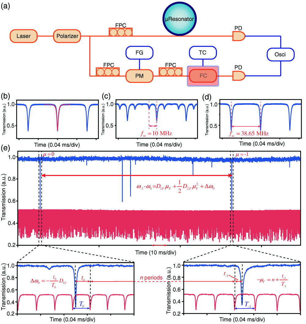
Fig. 1. (a) Schematic of the experiment setup. Orange lines denote optical paths, and blue lines represent electric cables. A tapered fiber is employed to couple the laser in and out of the microresonator. The fiber cavity is put on a silicone rubber heater, and both of them are kept in a thermal insulation box. Temperature is set as 50°C in the experiment. FPC, fiber polarization controller; FG, function generator; PM, phase modulator; TC, temperature controller; FC, fiber cavity; PD, photodiode. (b) Transmission spectrum of the fiber cavity without phase modulation. The red dashed line is Lorentz fitting for the resonance, and the fitting shows that the loaded Q of this fiber cavity mode is about 97 million. (c) Transmission spectrum of the fiber cavity when modulation frequency is 10 MHz. Two small dips in one FSR are caused by the resonance between sidebands and fiber cavity. (d) Transmission spectrum of the fiber cavity when modulation frequency is equal to one FSR of the cavity. In this situation, the transmission spectrum is almost the same as the one without phase modulation. (e) Measured microresonator transmission spectrum (blue) and etalon signal (red) of one microresonator FSR. The laser is scanned from short to long wavelength. Two small figures below the larger one are enlarged views.

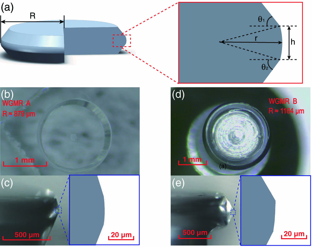
Fig. 2. (a) Geometric model of MgF2 microresonators. The left panel is an enlarged view of the microresonator boundary where light transmits. (b) Top view of WGMR A mounted on a glass plate. The measured main radius R is about 879 μm. (c) Front view of WGMR A. The right panel is the geometry used in FEM, which is obtained from the left panel by zooming in. In this model, r≈86  μm, h≈23  μm, θ1≈73°, θ2≈68°. (d) Top view of WGMR B mounted on a post. The measured main radius R is about 1164 μm. (e) Front view of WGMR B. The right panel is the geometry used in FEM, which is obtained from the left panel by zooming in. The arc area is rotated to make the model more coincident with the real one. In this model, r≈176  μm, h≈24  μm, θ1≈60°, θ2≈63°.

Fig. 3. (a) Electric field distribution of WGMR A with different azimuthal mode indices. (b) Simulation dispersion plot of Dint versus laser frequency of WGMR A. The resonator FSR acquired from the calculation is about 39.4 GHz. (c) Electric field distribution of WGMR B with different azimuthal mode indices. (d) Simulation dispersion plot of Dint versus laser frequency of WGMR B. The resonator FSR acquired from the calculation is about 29.5 GHz.

Fig. 4. Calculated D2/2π with different (a) r, (b) h, (c) θ1, and (d) θ of various azimuthal modes. In all calculations, the major radius of the microresonator is set as 879 μm, which is coincident with that of WGMR A.

Fig. 5. (a) Measurement dispersion Dint′ versus relative mode number μ. The measurement data are acquired from WGMR A. There is an obvious avoided mode crossing near the central mode. The right part of the plot is affected by several small mode crossings, which obviously decreases its ideality. (b) Binary fitting of measurement dispersion Dint′. The parameters obtained from this fitting are D2/2π=10.3  kHz, D2F/2π=43.5  mHz, a/2π=8.5  kHz, b/2π=−343  kHz. Adjusted R2 of the fitting is about 0.9991.

Fig. 6. (a) Transmission spectrum of measured mode of WGMR A with p=2. The measured FSR of WGMR A is around 39.6 GHz. (b) Mode spectrum corresponding to (a). Red points are plotted according to Eq. (5) after calibration. Blue line is acquired by parabolic curve fitting of the red points. Black dashed line denotes the calculation results of microresonator dispersion by FEM. The values of D2/2π obtained from measurement and simulation are given in the subplot, and the inset shows the results before calibration, which is the same as in Fig. 5(a). (c) Transmission spectrum of measured mode of WGMR B with p=2. The measured FSR of WGMR B is around 29.1 GHz. (d) Mode spectrum corresponding to (c). Left part of the spectrum is perturbed by several obvious mode crossings, while the ideality of the right part is influenced by some small mode crossings. (e) Transmission spectrum of measured mode of WGMR B with p=3. (f) Mode spectrum corresponding to (e). Five obvious avoided mode crossings appear on the spectrum, which may affect the dispersion measurement.

Fig. 7. (a) Transmission spectrum of measured mode of WGMR A with p=1. (b) Mode spectrum corresponding to (a). The spectrum is disturbed by many small mode crossings, which makes the dispersion derived from the data inaccurate. Graphic sign definitions are the same as in Fig. 6. (c) Transmission spectrum of measured mode of WGMR A with p=3. (d) Mode spectrum corresponding to (c). The spectrum is seriously affected by various small and large mode crossings. The parabolic curve fitting has a large deviation from the data points.