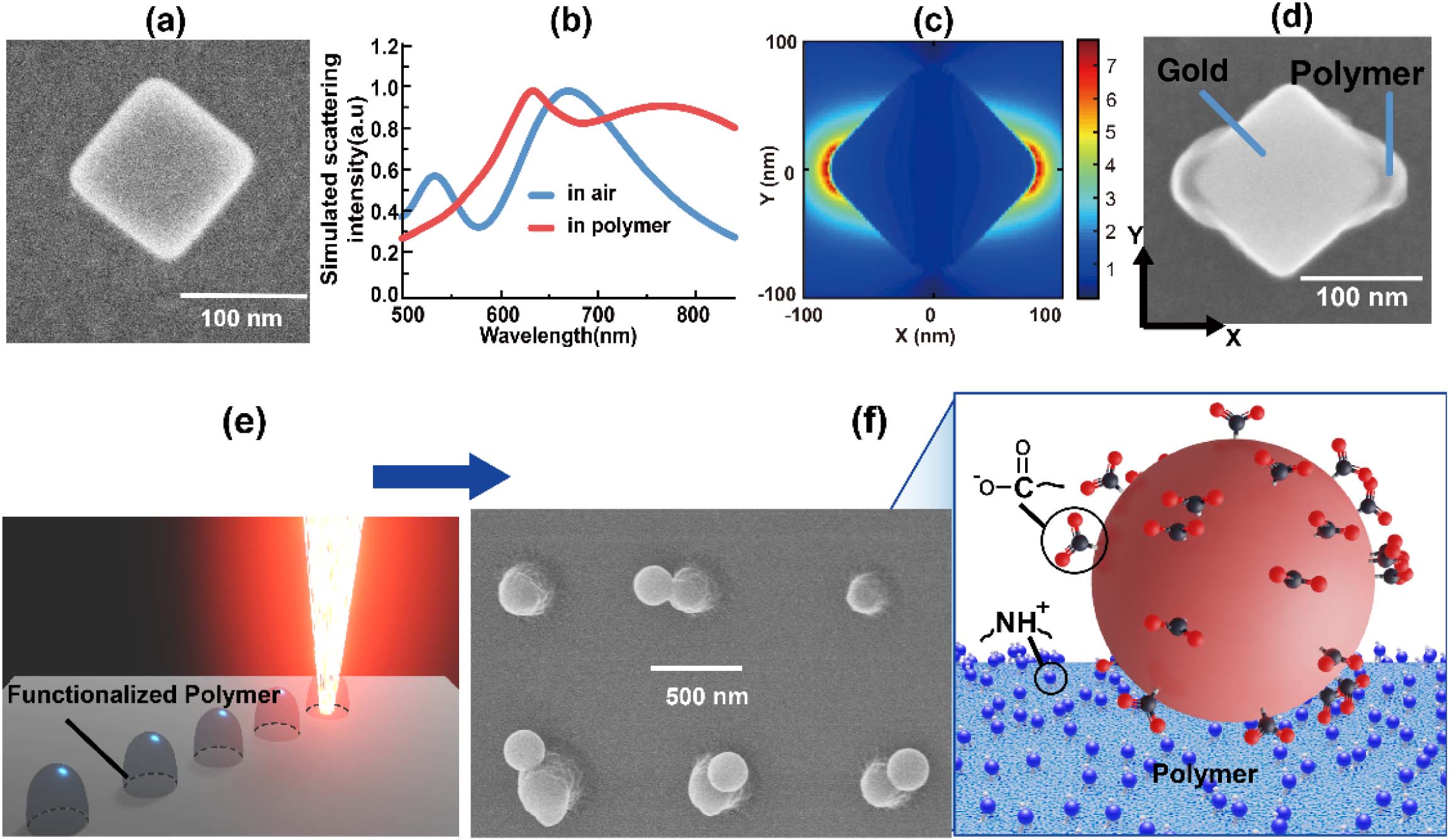
Fig. 1. GNC, nanoscale photopolymerization, and surface functionalization. (a) SEM image of a representative single GNC. (b) Calculated scattering spectrum of a single GNC of 125 nm, in air or photopolymer medium (refractive index=1.48), on ITO-coated glass substrate (40 nm thickness of ITO layer with refractive index of 2). (c) FDTD map (at the middle sectional plane of the cube, λ=780  nm) of the field modulus in the vicinity of the GNC illuminated with an X-polarized plane wave. (d) SEM image of the hybrid nanostructure resulting from two-photon polymerization (TPP) triggered by the field shown in (c). (e) Illustration of the photopolymerization of mixture of PETA monomer functionalized by amine. (f) Left: SEM image of polymerized dots whose surface contains amine group. After immersion in a solution of negatively charged functionalized fluorescent doped polystyrene spheres (200 nm diameter), the fluorescent spheres attached on four of the six polymer dots by electrostatic interaction. Right: schematic representation of the electrostatic interaction. NH⁺ represents the positively charged protonated amine group.

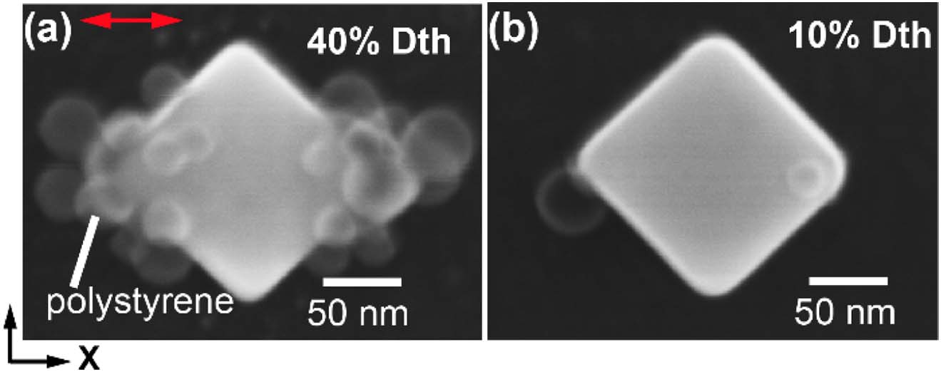
Fig. 2. SEM images of the hybrid FPSs attached nanostructures fabricated using energy dose of (a) 40% and (b) 10% of threshold during Step 1. The red arrow in (a) indicates the polarization direction of the excitation laser used for polymerization during Step 1.

Fig. 3. (a) Fluorescence spectrum measured from the hybrid FPSs–GNC shown in Fig. 2(a) using polarized green laser of 532 nm wavelength for excitation. A 650/150 nm bandpass filter is used to separate the fluorescent signal from the incident excitation. (b) Spectrum time trace, collected for 50s. (c) Definition of the polarization angle for excitation. (d) Fluorescence intensity as a function of the angle of incident polarization defined in (c).

Fig. 4. (a) Lifetime measurement of FPSs attached on hybrid polymer-cube fabricated by a dose of 40% Dth (orange) and 5% Dth (green). (b) Double-exponential fitting results of the lifetime of FPSs: fast decay component τ1, slow decay component τ2, and the coefficient a1 of fast decay component change as the average polymer thickness varies. (c) Weighted average lifetimes of FPSs change along the average distance between the metal surface and FPSs increased by decreasing the incident dose used to fabricate the hybrid GNC-based nanostructures. Dots of the same color represent hybrid nanostructures made with the same excitation energy dose. The pink area represents the variation range of the fluorescence lifetime of FPSs attached on polymer dots in the absence of gold particles. (d) Simulated average Purcell factor (P) of dipoles varies as the nano-polymer distribution changes by considering different incident energy doses and resulting average thicknesses. (e) and (f) Simulated field intensity (at Z=25  nm away from the bottom of the cube) of a hybrid FPS–GNC nanostructure fabricated individually using the energy dose of 40% Dth and 5% Dth. The excitation wavelength is set at 532 nm, and the incident light is polarized along X. The black dotted line depicts the FPS, and the white dotted line describes the contour of polymer.

Fig. 5. Use of the smart polymer to couple spherical CdSe/ZnS quantum dots with gold nanocubes. (a) AFM image of a hybrid nanosource made with an energy dose of 40% Dth. Attached QDs that result from Step 2 of the fabrication are clearly visible. (b) The spectrum time trace, signal collected during continuous 50 s. (c) Polarization sensitivity of the hybrid nanosource. (d) Measured lifetime for different hybrid nanosources with different polymer thicknesses. The red curve represents a reference lifetime decay of QDs attached on a polymer dot without a GNC nearby. (e) Double-exponential fitting results: evolution of fast and slow decay components τα, τβ, and coefficient α of a fast component as a function of the average polymer thickness. (f) Weighted lifetime as a function of the average polymer thickness that depends on the fabrication condition (proportion percentage in Dth energy used for near-field photo polymerization in Step 1).

Fig. 6. The process steps for fabricating hybrid FPS-attached cubes (FPS: fluorescent polystyrene sphere).

Fig. 7. Optical configuration to carry out two-photon polymerization.

Fig. 8. (a) Diameter distribution histogram of the fluorescent polystyrene spheres. (b) Excitation and emission spectra of polystyrene spheres measured separately by UV-visible Cary 100 spectrometer and fluorescence spectrophotometer. (c) Diameter distribution histogram of the QDs. The QDs are deposited on a glass substrate and then, after coating of a conducting layer, the QD sizes are measured under an SEM. Due to the existence of the conductive layer, the size of the measured QD is several nanometers larger than the real size of the QDs. (d) The absorption and emission spectra of the red QDs in toluene.

Fig. 9. More examples of hybrid FPS-attached GNCs. (a), (b) SEM images of the hybrid FPS-attached nanocubes fabricated using 40% Dth and 10% Dth, and the residence time of the FPS solution is 40 min. A 10 kV voltage is used for SEM observation. (c)–(g) FPS-attached nanocubes fabricated separately using 50% Dth, 40% Dth, 30% Dth, 10% Dth, and 5% Dth. The immersion time of the sample in the FPS solution is decreased to 10 min. A 1 kV voltage is used for SEM observation.

Fig. 10. AFM images of some hybrid GNCs with attached QDs, fabricated using incident doses from 80% decreasing to 10% of Dth (Step 1).

Fig. 11. Emission spectra from two hybrid FPS-attached GNCs fabricated using same parameters, and their exposure dose is 40% Dth. (a1) and (b1) The emission spectra from the first hybrid FPS-attached GNC when the polarization angle of the laser used for the excitation varies separately from 0 deg to 90 deg and 90 deg to 180 deg. (c1) The emission peak intensity changing trend. (a2), (b2), and (c2) The results from the second hybrid FPS-attached GNC.

Fig. 12. (a) SEM image of a hybrid nanocube without attaching any QDs/polystyrene spheres (fabricated using 50% Dth). (b) Mixed image, the original SEM image of the cube before exposure is superimposed to (a). (c) 40-degree tilted SEM image. (d) 3D height image measured by AFM of the same hybrid nanocube as (a). (d) 3D height image subtracted by the original cube’s height profile from (c), demonstrating the 3D polymer distribution.

Fig. 13. Average polymer thickness definition and assessment. (a) The whole hybrid cube-polymer structure is cut in the Z direction to get 20 slices of the cross-section. For each Z slice, a quadrant is sliced into N parts on average according to angle, and the intersection of the corresponding rays and the polymer profile is averaged to obtain the average elongation of the polymer under this Z slice. Finally, the polymer thickness of all slices in the Z direction is averaged to get the average polymer thickness. (b) The polymer elongations (l1, l2, l3) obtained by the three tangents when a quadrant is divided into three sections in the Z₁-slice, and then the average value of the three elongation rates of the polymer thickness of this slice.

Fig. 14. (a) First row shows an example of the lifetime from FPSs attached on a pure polymer dot without GNC nearby. Three kinds of fittings are used here: single-exponential fitting (gray line), double-exponential fitting (blue line), and triple-exponential fitting (orange line). The fitting results show that the single-exponential function can already achieve a good fitting result. The far-right image shows the histogram of the FPSs’ lifetime under a single-exponential fitting, and the green line represents the average value. For comparison, (b)–(d) show three examples of the lifetime from FPSs attached on the polymer lobes of a GNC.

Fig. 15. Example of the lifetime from QDs attached on pure polymer dot (a) without a GNC nearby and (b) with a GNC nearby. A single-exponential function is not enough to get a good fitting result while a double- or triple-exponential function can get a better fit. (c) Two failed attempts, by limiting the value range of τa (2–3), τβ (9–10) and τα (1–3), τβ (8–10) to attempt to use a similar τα, τβ in (a) to fit the decay curve.

Fig. 16. Fluorescence intensity from QDs attached on 2D flat functionalized polymer structure (see inset) with respect to the immersion time (min). The excitation laser is at 405 nm with a power of 2 μm, and the collection time is kept at 0.1 s. The left top small image (inset) is the dark-field image of the 2D flat polymer square.

Table 1. Calculated Average Polymer Thickness Using Different Percentages of Dth Doses