3D dynamic motion of a dielectric micro-sphere within optical tweezers

Jing Liu; Mian Zheng; Zhengjun Xiong; Zhiyuan Li

doi:10.29026/oea.2021.200015

Abstract

Known as laser trapping, optical tweezers, with nanometer accuracy and pico-newton precision, plays a pivotal role in single bio-molecule measurements and controllable motions of micro-machines. In order to advance the flourishing applications for those achievements, it is necessary to make clear the three-dimensional dynamic process of micro-particles stepping into an optical field. In this paper, we utilize the ray optics method to calculate the optical force and optical torque of a micro-sphere in optical tweezers. With the influence of viscosity force and torque taken into account, we numerically solve and analyze the dynamic process of a dielectric micro-sphere in optical tweezers on the basis of Newton mechanical equations under various conditions of initial positions and velocity vectors of the particle. The particle trajectory over time can demonstrate whether the particle can be successfully trapped into the optical tweezers center and reveal the subtle details of this trapping process. Even in a simple pair of optical tweezers, the dielectric micro-sphere exhibits abundant phases of mechanical motions including acceleration, deceleration, and turning. These studies will be of great help to understand the particle-laser trap interaction in various situations and promote exciting possibilities for exploring novel ways to control the mechanical dynamics of microscale particles.Known as laser trapping, optical tweezers, with nanometer accuracy and pico-newton precision, plays a pivotal role in single bio-molecule measurements and controllable motions of micro-machines. In order to advance the flourishing applications for those achievements, it is necessary to make clear the three-dimensional dynamic process of micro-particles stepping into an optical field. In this paper, we utilize the ray optics method to calculate the optical force and optical torque of a micro-sphere in optical tweezers. With the influence of viscosity force and torque taken into account, we numerically solve and analyze the dynamic process of a dielectric micro-sphere in optical tweezers on the basis of Newton mechanical equations under various conditions of initial positions and velocity vectors of the particle. The particle trajectory over time can demonstrate whether the particle can be successfully trapped into the optical tweezers center and reveal the subtle details of this trapping process. Even in a simple pair of optical tweezers, the dielectric micro-sphere exhibits abundant phases of mechanical motions including acceleration, deceleration, and turning. These studies will be of great help to understand the particle-laser trap interaction in various situations and promote exciting possibilities for exploring novel ways to control the mechanical dynamics of microscale particles.

Introduction

Micro-particles trapped in optical tweezers^{1, 2} can be utilized as carriers or handles that are biochemically linked to biological molecules. With nanometer accuracy of positioning and pico-newton precision of force measurement, optical tweezers offer an ideal platform to exert and measure the forces and torques on single bio-molecules or micro-particles^3-5. In 2018, A. Ashkin was awarded the Nobel Physics Prize for his contributions to invent the optical tweezers technology and promote its applications to biological systems. With the rapid development of optical tweezers technology, simple manipulation of particles is no longer sufficient to support either scientific research or industry demands. For example, the first necessary step for statistically analyzing the trajectory of a trapped particle is to track the particle position accurately. This is often achieved by acquiring a video^{6, 7}, stereomicroscopy⁸, V-shaped micro-mirrors⁹ of the particle, or other visualization techniques including position sensitive detection¹⁰ and quadrant photodiode detection¹¹, which monitors via detecting the backscattering signal or transmitting signal. In fact, these experimental techniques are limited by sampling rate and in 3D imaging applications. Up to now, it is still very hard to track the 3D trajectory of a micro-particle with high precision. Currently, numerical researches^{12, 13} are conducted to investigate the optical force exerted on trapped particles. However, the detailed dynamics of a particle stepping into a laser trap^{14, 15} is still an area rarely studied.

This situation inspires us to think of an idea to drive a particle into a steady state by a focused laser beam illuminating it. As it is very difficult or even impossible to determine trapping probabilities through real-world experiments due to the large parameter space (including, for example, the initial states of particles position, velocity, etc.), we have developed a computational framework in which trapping probabilities can be determined easily through numerical simulations. Simulation involves calculating the optical forces and torques, non-optical forces and torques, and combining these components to calculate the overall dynamics of the particle.

A significant concern is how to calculate the optical force and torque of mesoscopic particles. There are two main types of approaches: namely ray optics method and electromagnetic scattering method. In terms of the computational resources and time to solve the dynamic process, the ray optics method has advantages over electromagnetic approaches such as finite-difference time-domain (FDTD) method¹⁶ or T-matrix method^{17, 18}. Taking the widely used method of FDTD as an example, the simulation area is needed to be 5 μm × 5 μm × 5 μm for a 3 μm diameter micro-particle. When the micro-particle is far away from the laser trap, the simulation area is even larger. Furthermore, a complete dynamic process involves thousands or even millions of trajectory points, and it is needed to calculate all mechanical quantities (forces and torques) at each point in order to determine the next point of the trajectory by solving electromagnetic fields in a large 3D space. With FDTD or T-matrix method, the time consumption at each point is at the scale of minutes or even hours. Therefore, the solution to a single set of dynamic process costs days or even months. This is a computational burden too heavy which exceeds the capacity of common computers. As for the semi-analytical ray optics method, the time cost is at the scale of millisecond to implement the optical force and torque calculation of each trajectory point, which makes this method a good compromise between clarity and exactness in many situations^{19, 20}. Therefore, we employ the ray optics method to obtain the optical force and torque of the micro-particles in the optical tweezers.

In this paper, we utilize the ray optics theory to calculate optical forces and optical torques. Then, with the influence of viscosity forces and torques taken into account, we numerically analyze the 3D dynamic process of dielectric micro-spheres in optical tweezers on the basis of Newton mechanical equations. In addition, the supplementary videos show the 3D dynamic process of the micro-sphere particles with different initial states of particle positions and velocities. These studies can be valuable to understand experiments that have been performed, to predict the results of potential experiments, or to explore the mechanical dynamics of trapped particles that are not accessible experimentally. Furthermore, these studies can open up opportunities to explore possible applications based on controlling the dynamics of a particle in the optical tweezers.

Theory and formulas for solution of mechanical dynamics

Investigating the dynamic process of a micro-sphere can be divided into three steps. The first step is to calculate the optical force and torque, the second step is to calculate the non-optical force and torque, and the third and final step is to numerically solve the Newton mechanical equations. This section describes the theory and formulas for solving the dynamic process of the micro-sphere in optical tweezers systematically.

Calculation of optical force and torque

The schematic of the optical tweezers considered in this work and the coordinate system used in our calculation is shown in Fig. 1(a). The center of the optical tweezers, point “O”, is set as the coordinate origin. The collimated Gaussian beam at a wavelength $λ = 1064 nm$ propagates along the z-axis and is focused by a high numerical aperture (NA=1.4) objective. We implement the procedures and methods developed in ref.²¹ to calculate the optical force ( $F_{optical} = [F_{x}, F_{y}, F_{z}]$ ) and the optical torque ( $τ_{optical} = [τ_{x}, τ_{y}, τ_{z}]$ ) of a dielectric micro-sphere in optical tweezers when the micro-sphere with radius $r_{s}$ moves around the focus point along the x-, y-, and z-axes, respectively. The initial parameters are as follows. The surrounding medium is water with a refractive index $n_{1} = 1.33$ , the dielectric micro-sphere has a refractive index of $n_{2} = 1.6$ and radius $r_{s} = 1 μ m$ , and the laser power is $P = 10 mW$ . 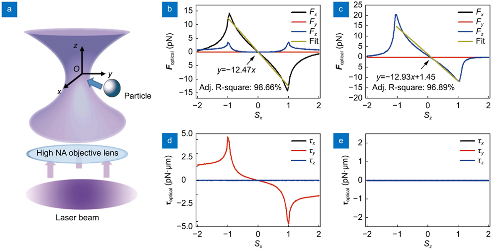In Figs. 1(b)−1(d), we display the calculated optical force and torque as a function of the position along the x− and z− axes of the micro-sphere around the identified equilibrium position. The results analysis about the initial parameters of the micro-sphere in the y-axis can be deduced from that in the x-axis. Due to the symmetry of the x− and y− axis directions, the curve $F_{optical} \sim S_{y}$ is the same to the curve $F_{optical} \sim S_{x}$ , and the curve $τ_{optical} \sim S_{y}$ is mirror symmetrical to the curve $τ_{optical} \sim S_{x}$ . In addition, to characterize the optical trapping probability, we need to measure the trap stiffness $κ = [κ_{x}, κ_{y}, κ_{z}]$ . If the particle is not far away from the trap center (so-called Hookean region, $| Δ S / r_{s} | ⩽ 1$ ), the optical force exerted on the particle is directly proportional to the displacement $Δ S = [Δ S_{x},$ $Δ S_{y}, Δ S_{z}]$ from the equilibrium position $S = [S_{x},$ $S_{y}, S_{z}]$ , i.e. $F_{optical} = κ_{x} Δ S_{x} \hat{x} + κ_{y} Δ S_{y} \hat{y} + κ_{z} Δ S_{z} \hat{z}$ . Through linear fitting of the data in Hookean region, the trap stiffness coefficients in x− andz− axes are calculated and they are $κ_{x} = - 12.47 pN/ μ m$ and $κ_{z} = - 12.93 pN/ μ m$ , respectively. The yellow line in Figs. 1(b) and 1(c) characterizes the trap stiffness. In Fig. 1(d), the micro-sphere only experiences the torque in the y-axis ( $τ_{y}$ ) when it moves along the x-axis direction. And it can be inferred that there is no torque acting on the micro-sphere when it moves along the z-axis because of the structure symmetry, as shown in Fig. 1(e).

Figure 1.(a) Schematic of basic optical tweezers. A single laser beam is focused by a high numerical aperture objective lens to form a stable optical trap for microscale particle. (b) and (c) illustrate the calculated optical force acting on a micro-sphere when it moves along the x-axis and z-axis, respectively, in the optical tweezers at the laser power P = 10 mW. Here, the two most important features of optical tweezers are shown: the maximum reverse axial force that characterizes the strength of the trap, and spring constants (the slope of the fit line). (d) and (e) display the calculated optical torque acting on a micro-sphere when it moves along the x-axis and z-axis, respectively.

Calculation of non-optical force and torque

In general, all the particles experience drag forces coupled with a rapid fluctuation force, which is the result of frequent and numerous collisions with surrounding liquid molecules and the physical origin of famous Brownian motion. The drag force acting on the particle is obtained by the expression

1 $F_{drag} = - γ \cdot v,$

where $γ$ is the viscous drag coefficient and $v$ is the particle velocity relative to the surrounding liquid. For a spherical bead, $γ$ is expressed by the Stokes equation,

2 $γ = 6 π η r_{s},$

where $η$ is the fluid viscosity, $0.89 \times 10^{- 3} Pa \cdot s$ for water at room temperature and $r_{s}$ represents the radius of the micro-sphere. Meanwhile, the drag torque can be calculated as follows,

3 $τ_{drag} = 8 π r_{s}^{3} η ω,$

here, $ω$ is the angular velocity of the spherical particle.

Moreover, the gravity $G$ and buoyancy $F_{buoy}$ acting on the micro-sphere are written using the density of the micro-sphere and the density of water, $ρ_{s} = 1.03 \times$ $10^{3} {kg/m}^{3}$ and $ρ_{w} = 1.0 \times 10^{3} {kg/m}^{3}$ respectively, the radius of the micro-sphere $r_{s}$ , and the gravitational acceleration $g$ ,

4 $G = - \frac{4}{3} π r_{s}^{3} ρ_{s} g,$

5 $F_{buoy} = \frac{4}{3} π r_{s}^{3} ρ_{w} g .$

It is noted that the direction of the forces $G$ and $F_{buoy}$ is along the z-axis. Therefore, their resultant forces pass through the center of mass, which provides no torque to the micro-sphere.

Solution of Newton mechanical equations

In order to implement numerical analysis over the dynamic process, the Newton mechanical equations are exploited to accurately model the dynamic parameters of the trapped micro-sphere in the optical tweezers. The equation of the micro-sphere translational motion^22-24 can be written as

6 $m \ddot{r} = F_{optical} (r, P) + F_{drag} (v) + G + F_{buoy},$

where $r$ is the micro-sphere position with respect to the laser center; $m$ is the mass of the micro-sphere.

Similarly, the equation of the micro-sphere rotational motion²¹ can be expressed by

7 $I ϕ = τ_{optical} (ϕ, P) + τ_{drag} (ω),$

here, $I = 2 / 5 m r_{s}^{2}$ represents the moment of inertia of the micro-sphere, and $ϕ$ is the initial angular of the micro-sphere.

As Eqs. (6) and (7) cannot be solved analytically, the Runge-Kutta methods, a family of implicit and explicit iterative methods, are used in temporal discretization for the approximate solutions of ordinary differential equations (ODEs). One of the above methods, the fourth-order Runge-Kutta method (RK4 method) is utilized. This method has successfully been employed for solving the ODEs^25-27. The second-order differential equation Eqs. (6) and (7) each can be converted to two coupled first-order equations respectively,

8 $\dot{v} = \frac{F_{optical} (r, P) + F_{drag} (v) + G + F_{buoy}}{m} = a (r, v),$

9 $\dot{r} = v .$

And

10 $\dot{ω} = \frac{τ_{optical} (ϕ, P) + τ_{drag} (ω)}{I} = α (ϕ, ω),$

11 $ϕ = ω .$

Since the time step has a direct effect on the number of iterations required for running a simulation, we have to choose an appropriate time step size. The characteristic time scale of our entire model is given by the relaxation time $m / γ \sim 27 ns$ . In our computations, the numerical integration time step $δ t$ is set to 10 $ns$ , such that $δ t < m / γ$ . Choosing such a small $δ t$ provides an opportunity to observe interesting non-equilibrium behavior in the simulation.

The recursive algorithm for the classical RK4 method can be written as follows. Taking a particular position step $r_{i}$ for an example, the mechanical dynamics evolution can be written as

12 $f_{a 1} = a (r_{i}, v_{i}),$

13 $f_{v 1} = v_{i},$

14 $f_{a 2} = a (r_{i} + δ t / 2 \cdot f_{v 1}, v_{i} + δ t / 2 \cdot f_{a 1}),$

15 $f_{v 2} = v_{i} + δ t / 2 \cdot f_{a 1},$

16 $f_{a 3} = a (r_{i} + δ t / 2 \cdot f_{v 2}, v_{i} + δ t / 2 \cdot f_{a 2}),$

17 $f_{v 3} = v_{i} + δ t / 2 \cdot f_{a 2},$

18 $f_{a 4} = a (r_{i} + δ t / 2 \cdot f_{v 3}, v_{i} + δ t / 2 \cdot f_{a 3}),$

19 $f_{v 4} = v_{i} + δ t / 2 \cdot f_{a 3} .$

The position and velocity of the micro-sphere in the next integration time interval are solved as

20 $r_{i}_{+ 1} = r_{i} + (δ t / 6) \cdot (f_{v 1} + 2 f_{v 2} + 2 f_{v 3} + f_{v 4}),$

21 $v_{i}_{+ 1} = v_{i} + (δ t / 6) \cdot (f_{a 1} + 2 f_{2 a} + 2 f_{a 3} + f_{a 4}) .$

Similarly, the mechanical evolution of the remaining physical values $ω_{i + 1}$ , $ϕ_{i + 1}$ follows the same procedures described above.

With the above iterative methods, we can obtain the dynamic parameters $r (t)$ , $v (t)$ , $ω (t)$ , and $ϕ (t)$ of the micro-sphere in the optical tweezers with high precision and retrieve every details of the micro-sphere mechanical motion in 3D space. These results can be interpreted in a direct correspondence to the time-space dynamic process. Note in particular that this micro-sphere simulation framework is applicable to either a continuous or a discrete optical force.

Dynamics of micro-sphere at different initial positions

On the basis of the above simulation framework, we set a series of initial parameters for the micro-sphere in the optical tweezers, and go further to theoretically draw a picture of its dynamics of mechanical motion. At first, we choose a special initial position of the micro-sphere close to the laser center. This special initiation indicates a high trapping probability, which can help find out whether the simulation framework agrees with experimental results quantitatively or not.

The initial parameters are as follows: the initial position $r_{0} = [0,0,1] μ m$ , the initial velocity $v_{0} =$ $[0,0,0] μ m/s$ , the initial angular displacement $ϕ_{0} = [0,0,0] rad$ , and the initial angular speed $ω_{0} = [0,0,0] rad/s$ . In addition, the gravity and buoyancy of the micro-sphere are $G = - 4.27 \times 10^{- 2} pN$ and $F_{buoy} = 4.11 \times 10^{- 2} pN$ , respectively. The simulated numerical results of trajectory, velocity, angular velocity, and optical force of the micro-sphere in the optical tweezers are plotted in Fig. 2 for the laser power of 10 mW. In Fig. 2(a), which illustrates the temporal evolution of the micro-sphere position, it can be seen that the micro-sphere goes straight to the equilibrium position, and finally is tightly trapped in optical tweezers. On the other hand, according to Fig. 2(b), which displays the temporal evolution of micro-sphere velocity, in the beginning, the micro-sphere is in the stationary state. Then it accelerates to a high velocity $v_{\max_z} = - 671.79 μ m/s$ in an extremely short time (below one microsecond), followed by a modest deceleration until a stable capture is reached in a time scale of several milliseconds. Due to the radial symmetrical structure of the micro-sphere and optical tweezers, the micro-sphere only experiences the optical force along the z-axis, $F_{z}$ [shown in Fig. 2(d)]. Moreover, due to the radial symmetrical force exerted on the micro-sphere, no torque exists to supports its rotation [displayed in Fig. 2(c)]. The data in Figs. 2(c) and 2(d) are consistent with the physical analysis and naive expectation. The stable position is [0,0,0.085]. It shows that the trapping potential well center for the micro-sphere particle is in the optical axis, i.e., the z-axis, and slightly shifting forward (0.085 $μ m$ ) away from the laser beam focus center without the particle, due to the refraction effect of the particle against the laser beam. Besides, the micro-sphere spends about 0.008 second on reaching the stable position, which agrees well with the results reported in ref.²⁸.

Figure 2.The dynamic process of the micro-sphere in an optical tweezers. Plots of the (a) position, (b) velocity, (c) angular velocity, and (d) optical force versus time under the initial condition of r₀=[0,0,1] μm, v₀=[0,0,0] μm/s, ϕ₀=[0,0,0] rad, and ω₀=[0,0,0] rad/s.

Having confirmed the accuracy and efficiency of the numerical methods, we proceed to estimate the trapping probabilities by systematically performing simulation at random initial positions and velocities in the parameter space. This greatly helps on judging whether the micro-sphere can be trapped stably and efficiently in the optical tweezers. In the following, we first consider the dynamics of microsphere with different initial positions but with fixed initial zero velocity. We compare the motion trajectories of the micro-sphere when it is set at different initial positions in the optical tweezers. Apart from the initial positions, the rest parameters are as follows, the initial velocity $v_{0} = [0,0,0] μ m/s$ , the angular displacement $ϕ_{0} = [0,0,0] rad$ , and the angular speed $ω_{0} = [0,0,0] rad/s$ .

In the first case, the initial position of the micro-sphere is set to be located on the horizontal plane crossing the trapping center and moving along the x-axis, so that the coordinate on the y- and z- axes is given by $r_{0 y} = 0 μ m$ and $r_{0 z} = 0.085 μ m$ . Figure 3(a) shows the temporal evolution of the x-directional trajectories of the micro-sphere at different initial positions in the x-axis with $r_{0 x} =$ 0.5, 1.0, 1.5, 1.8, 1.9, and 2.0 $μ m$ , respectively. When the initial position is within the Hookean region ( $| r_{0 x} | ⩽ 1.0 μ m$ ), the micro-sphere experiences a strong restoring force, as shown in Fig. 1(b). It rapidly falls into the laser center, then finally locates at the equilibrium position. Interestingly, even though the initial position is out of the Hookean region ( $1.5 μ m ⩽ | r_{0 x} | ⩽ 1.9 μ m$ ), the micro-sphere still can be trapped in the optical tweezers. This phenomenon is due to the fact that the micro-sphere experiences the synergetic effect between the x-axis optical force $F_{x}$ and the z-axis optical force $F_{z}$ . At this time, the force $F_{z}$ plays a very important role in dominating the final state of the micro-sphere motion. For clear illustration, we plot the detailed pictures of the trajectory, the optical force and the viscous drag force, and the resultant force $F_{sum}$ ( $F_{sum} = F_{optical} + F_{drag} + G + F_{buoy}$ , which are the same in all context) of the micro-sphere placed at $r_{0 x} =$ 1.9 $μ m$ , and display them in Figs. 3(b), 3(c) and 3(d), respectively. In Fig. 3(b), the micro-sphere moves towards the laser center in the x-axis direction, while away from that in the z-axis direction in the early stage ( $T ⩽ 0.015 s$ ). In the intermediate stage ( $0.015 s ⩽ T ⩽ 0.045 s$ ), the micro-sphere moves slowly in the z-axis direction, and keeps on moving close to the laser center in the x-axis. In the last stage, the micro-sphere overcomes viscous resistance and slowly reaches the Hookean region ( $r = [0.68,0,0.73] μ m$ ) at the time $T = 0.046 s$ , then goes straight to the equilibrium position with a great speed. In Fig. 3(c), the plot of the optical force $F_{optical} = [F_{x}, F_{y}, F_{z}]$ and the drag force $F_{drag} = [F_{drag_x}, F_{drag_y}, F_{drag_z}]$ exerted on the micro-sphere also helps us to understand its dynamic process. In the early stage, the negative force $F_{x}$ pulls the micro-sphere into the trap, while the positive force $F_{z}$ pushes it away. In the intermediate stage, the value of the force $F_{z}$ is low so that the micro-sphere moves slowly in the z-axis. More importantly, the direction of the force $F_{z}$ has changed from the positive zdirection to the negative zdirection, which indicates the capture of the micro-sphere. In the whole process, the drag force $F_{drag}$ opposes its motion, and varies with the velocity of the micro-sphere. On the other hand, in Fig. 3(d), the resultant force $F_{sum}$ are helpful in understanding the motion of the micro-sphere. For example, the resultant force is so small in the intermediate stage compared with other forces, and the micro-sphere moves very slowly correspondingly. When $r_{0 x} = 2.0 μ m$ , the optical force, drag force, and the resultant force over time are calculated and displayed in Figs. 3(e) and 3(f), respectively. The direction of the force $F_{z}$ always points to the positive zaxis, so that it pushes the micro-sphere away from the laser center. Meanwhile, the force $F_{x}$ is too small to pull the micro-sphere back to the trap center. As the micro-sphere moves away from the laser center, the resultant force approaches zero. Therefore, this initial position will not lead to successful trap of the micro-sphere.

Figure 3.Mechanical motion dynamics of the micro-sphere at different initial positions in the horizontal trapping plane. (a) The x-directional trajectories of the micro-sphere at different initial positions in the x-axis in the optical tweezers with r_0x=0.5, 1.0, 1.5, 1.8, 1.9, and 2.0 μm. (b)−(d) display the temporal evolution of the x- and y- and z- directional trajectory, optical force, drag force, and resultant force, respectively, when the micro-sphere is set at the initial position r_0x=1.9 μm. (e) and (f) display the temporal evolution of the optical force and the drag force, and the resultant force, respectively, when r_0x=2.0 μm.

Figure 4 shows the corresponding 3D trajectories of the micro-sphere. The color bar represents the time. This picture can illustrate the temporal evolution of the micro-sphere mechanical motion in 3D space. Moreover, these 3D dynamic processes of the micro-sphere are better visualized in Supporting Information (SI) Video S1. In Fig. 4 and Video S1, it is obvious that the micro-sphere does not follow the shortest straight path to move to the stable position. Besides, the complexity of its trajectory increases as the initial position is located farther away from the laser center. When the micro-sphere is set at $r_{0 x} \leq 1.5 μ m$ , it moves fast along the corresponding trajectory, and takes less than 0.015 second to reach the stable position. While at $r_{0 x} = 1.8 μ m$ or $1 .9 μ m$ , its trajectory has been described in Fig. 3(b). As observed in Video S1, the micro-sphere exhibits abundant types of mechanical motions, including acceleration, deceleration, and turning. However, these short dynamic processes are easily overlooked in experiments. With $r_{0 x} = 2.0 μ m$ , in a period of 0.06 second, the micro-sphere also undergoes many motion phases as in other initial positions, but without a successful capture in the end. If the micro-sphere is utilized as a handle linked to single bio-molecule, these specific motion details can provide key information on the dynamic process of the attached single bio-molecule.

Figure 4.The 3D trajectories of the micro-sphere in the optical tweezers at different initial positions in the x-axis with r_0x= 0.5, 1.0, 1.5, 1.8, 1.9, and 2 μm.

In the second case, the initial position of the micro-sphere is set to be located at the z-axis with $r_{0 x} = 0 μ m$ , $r_{0 y} = 0 μ m$ . Fig. 5(a) shows the temporal evolution of the z-directional trajectories of the micro-sphere at different initial positions in the z-axis with $r_{0 z} =$ −2.0, −1.5, −1.0, −0.5, 1.0, 1.4, 1.6, 1.7, 1.75, and 1.9 $μ m$ , respectively. The corresponding dynamic motions are shown in Supplementary information Video S2. Due to the symmetry of micro-sphere and optical tweezers, the optical force acting on the micro-sphere always has $F_{x} = 0$ and $F_{y} = 0$ . Therefore, the micro-sphere experiences the optical force along the z-axis only and thus also moves along the z-axis only. In this situation, the forces $G$ and $F_{buoy}$ also apply a little bit of work. When $- 2 μ m ⩽ r_{0 z} ⩽ 0 μ m$ , the required equilibrium time, which is the time for the trapped micro-sphere to reach its equilibrium position, is positively correlated with the distance from the trap center. When $0 μ m ⩽ r_{0 z} ⩽ 1.0 μ m$ , the micro-sphere experiences a strong propulsion force, rapidly falls into the laser center, and eventually locates at the equilibrium position. When $1.4 μ m ⩽ r_{0 z} ⩽ 1.75 μ m$ , the micro-sphere is captured in the end but the situation differs from above. As a reference, the sketches of the optical force and drag force, and the resultant force varying over time are shown in Figs. 5(b) and 5(c) when $r_{0 z} = 1.7 μ m$ . In the initial stage, the micro-sphere moves slowly, which is primarily due to the small resultant force. While entering into the Hookean region, it rapidly falls into the trap because of the huge restoring optical force. Eventually, it will stop due to the drag force. When $r_{0 z} ⩾ 1.9 μ m$ , the direction of the optical force $F_{z}$ points to the positive zdirection, as shown in Fig. 1(c), and it pushes the micro-sphere away from the laser center. Clearly, this initial position will not lead to successful trap of the micro-sphere.

Figure 5.Mechanical motion dynamics of the micro-sphere at different initial positions along the optical axis. (a) The z-directional trajectories of the micro-sphere at different initial positions in the z-axis in the optical tweezers with r_0x=−2.0, −1.5, −1.0, −0.5, 1.0, 1.4, 1.6, 1.7, 1.75 and 1.9 μm. (b) and (c) The sketches of the optical force and the drag force, and the resultant force over time, respectively, when the micro-sphere is set at the initial position r_0x=1.7 μm.

Dynamics of micro-sphere at different initial velocities

In this part, we consider, calculate, and display the motion trajectories of micro-sphere when it is set at different initial velocities. Similar to the past sections, we have listed the initial parameters, the initial position $r_{0} = [0,0,0] μ m$ , the angular displacement $ϕ_{0} = [0,0,$ 0] rad, and the angular speed $ω_{0} = [0,0,0] rad/s$ . In the first case, the micro-sphere is set to be located at the laser trap center and has initial velocity components of $v_{0 y} = 0 μ m/s$ and $v_{0 z} = 0 μ m/s$ .

The corresponding 3D trajectories and dynamic motions of the micro-sphere at different x-directional initial velocities with $v_{0 x} =$ 100, 1 $\times 10^{4}$ , 1 $\times 10^{6}$ , 5 $\times 10^{6}$ , 7.5 $\times 10^{6}$ , 7.75 $\times 10^{6}$ , and 8 $\times 10^{6}$ μm are shown in Fig. 6 and Supplementary information Video S3. In the initial stage, the micro-sphere with an initial velocity will continue to move and reach a new position because of the inertia. According to the equation $F_{drag} = γ \cdot v$ , the higher speed, the larger viscous force. Thus, the velocities decrease rapidly. Additionally, it moves under a variety of forces, including the optical force, the drag force, the gravity, and the buoyance. In the following processes, its motion is similar to the situations with the different x-axis initial positions in Fig. 4. Moreover, the x-directional initial velocity is essential to the trapping probabilities and the capture time. When $v_{0 x} ⩽ 5 \times 10^{6} μ m/s$ , it takes less than 0.01 second for the micro-sphere to reach the steady state. While $v_{0 x} = 7.75 \times 10^{6} μ m/s$ , it takes about 0.06 second. When $v_{0 x} ⩾ 8 \times 10^{6} μ m/s$ , the micro-sphere is hard to be captured. The experience gained via this systematical study is particularly useful in determining the initial velocity of a particle in the liquids required for the particle to be successfully trapped.

Figure 6.The 3D trajectories of the micro-sphere at different initial velocities in the x-axis in the optical tweezers with v_0x=100, 1×10⁴, 1×10⁶, 5×10⁶, 7.5×10⁶, 7.75×10⁶, and 8×10⁶ μm/s.

Dynamics of micro-sphere with general initial mechanical conditions

In this part, we go further to investigate the motion trajectories of the micro-sphere in more general initial conditions of positions and velocities. The initial parameters are set as follows: the angular displacement $ϕ_{0} = [0,0,0] rad$ , the angular speed $ω_{0} = [0,0,0] rad/s$ , the position is located at x-axis ( $r_{0} = [1,0,0] μ m$ ), while the velocity $v_{0}$ is parallel to the z-axis.

Figure 7(a) shows the 3D trajectories of the micro-sphere at different z-directional initial velocities with $v_{0 z} =$ 1 $\times 10^{6}$ , 5 $\times 10^{6}$ , 6 $\times 10^{6}$ , and 6.5 $\times 10^{6}$ $μ m/s$ , respectively. In addition, the initial position is marked with a pentagon. The corresponding dynamic motions can be observed in Supplementary information Video S5. Although the optical force exerted on the micro-sphere at the initial position is $F_{optical} = [- 11.9,0,5.3] pN$ , the micro-sphere still moves upward with the initial z-directional velocities and reaches a new position because of the inertia. When $v_{0 z} = 1 \times 10^{6} μ m/s$ , the micro-sphere just moves up a little bit. After that, it reaches the stable position rapidly, in less than 0.01 second. When $5 \times 10^{6} μ m/s ⩽ v_{0 z} ⩽ 6 \times 10^{6} μ m/s$ , the micro-sphere moves towards the positive x direction while moving downwards concurrently. Later, it makes a large-angle turning. Specifically, the micro-sphere changes its motion direction, shifts in the negative x direction while moving downwards, and approaches the equilibrium position. Taking $v_{0 z} = 6 \times 10^{6} μ m/s$ as an example, we have calculated and plotted the optical force and drag force, and the resultant force of the micro-sphere in Figs. 7(b) and 7(c), respectively. As is well known, both the magnitude and direction of the optical force $F_{x}$ vary with its location. The key to the turning is that the direction of the force $F_{x}$ is reversed when $T = 0.016 s$ . After that, the micro-sphere moves slowly along the trajectory for about 0.02 seconds, and then rushes into the stable position. When $v_{0 z} = 6.5 \times 10^{6} μ m/s$ , although the micro-sphere moves towards the negative zdirection in the early stage, it keeps heading in the positive x direction in the whole process. As a result, it is hard to successfully trap the micro-sphere in this situation.

Figure 7.(a) The 3D trajectories of a micro-sphere at different initial velocities in the z-axis with v_0x=1×10⁶, 5×10⁶, 6×10⁶, and 6.5×10⁶ μm/s, when the initial position is r_0x=[1,0,0] μm. The plots of (b) the optical force and drag force, and (c) the resultant force over time of the micro-sphere when v₀=[6.5 × 10⁶,0,0] μm/s, and r_0x=[1,0,0] μm.

In the above discussions, we just list several special cases to describe the micro-sphere trapping probabilities. Nevertheless, there will be various combinations of initial parameters to characterize the motions of the micro-sphere in the optical tweezers. In any of these cases, the theoretical and numerical method proposed in this paper can give a reasonable solution and calculation of the mechanical motion dynamic process, and also explain how and why the micro-sphere moves, whether or not, how and why it can be trapped. It should be noted that the initial angular displacement and angular speed have not been discussed or analyzed in the present work. It is mainly because the optical torque is very small as shown in Fig. 1(d)] while the drag torque is relatively very large ( $τ_{drag} = 8 π r_{s}^{3} η ω$ ). Thus, the rotation state of the micro-sphere will not last long and is very hard to be observed in experiments. There is still a critical problem that in the microscopic world, due to the random bombardment of the water molecules, the Brownian motions of particles become increasingly significant with the decreasing size of the particles. In terms of the trapped micro-sphere, the Reynolds number of fluid is rather small, which is much less than 1, therefore the viscous forces rather than Brownian force dominate its dynamic process.

Through simulating the dynamic process, the change of the relevant physical parameters of the micro-sphere [ $r (t), v (t), ϕ (t), ω (t), F_{optical} (t), F_{drag} (t), F_{sum} (t)$ ] over time are very clear. This can help us understand, and even predict the results of experiments such as trapping probabilities, balance time, the maximum velocity, etc. Meanwhile, the above method can also be utilized in analyzing the dynamic process of a complicated-geometry particle in complicated-structure beams, which creates new possibilities for constructing mixed laser beams to generate various motions for microscale particles.

Conclusions

In summary, we have proposed a method based on semi-analytical ray optics model to visualize the dynamic process of a dielectric micro-sphere in optical tweezers. This approach allows for a fast calculation of optical force and torque exerted upon micro-sphere by focused laser beam with reasonable accuracy and makes it possible to simulate the whole mechanical motion trajectory and process of the particle under Newton’s law. We discuss the trapping probabilities of the micro-sphere at the different initial positions or velocities along the x- and z- axes respectively. It has been found that, unexpectedly, the particle still has the possibility to be trapped by the optical tweezers even if its position is out of the Hookean region. In contrast, the micro-sphere with a large initial velocity will not necessarily be trapped even if its position is in the Hookean region.

On the other hand, even in simple optical tweezers, the dielectric micro-sphere exhibits abundant phases of mechanical motions, including acceleration, deceleration, and turning. Solution and analysis of the 3D microscale particle dynamic process within optical trapping is essential for understanding various mechanisms for engineering the light-matter mechanical interactions, the mechanical motion behavior of molecules or micro-particles in liquid, as well as the biophysics and biochemistry of macromolecules and cells. These dynamics will facilitate the investigation of the single-molecular kinematics, the complex motions of diverse particles and so on. In addition, this method opens up a new way to promote optimal external control in various applications, including molecular winding, nanoparticles sorting, and in vivo manipulations. However, this method is still not mature enough. In the future, we shall perfect the theory of the micro-particle dynamics, and take more factors into consideration, such as the Brownian motion of particles, the change of the viscous drag coefficient (due to the action of the cover glass), the physical characteristics of the particles (shape, radius, refractive index), etc.

References