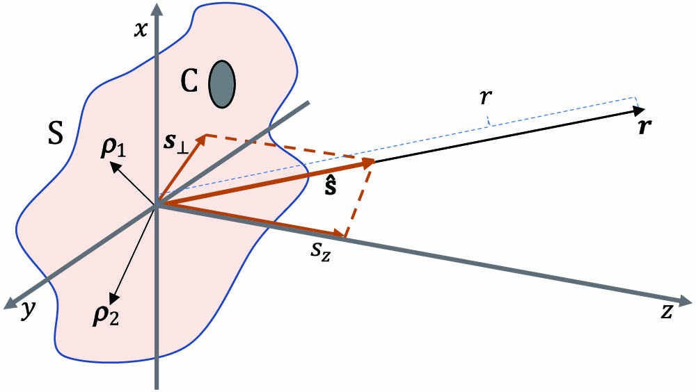
Fig. 1. Geometry and notation relating to a quasihomogeneous planar source with an emitting area S far larger than the effective coherence area C, and far-field radiation from such a source. Here ρ1 and ρ2 represent two arbitrary points in the source plane. The unit vector s^=(s⊥,sz) refers to an arbitrary position r=rs^ at a distance r in the far zone.

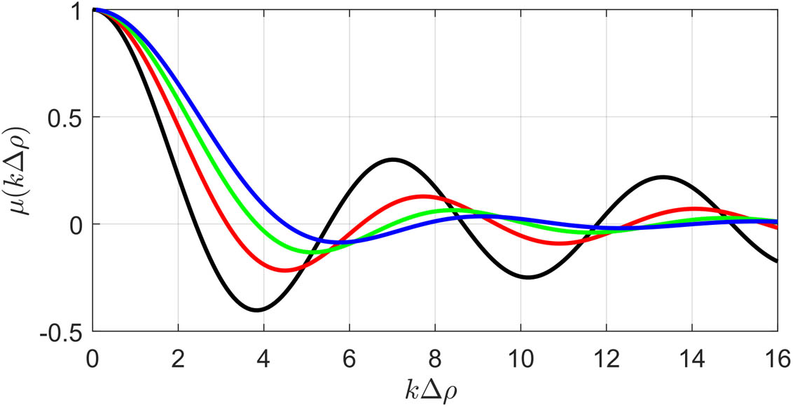
Fig. 2. Plots of the complex degree of coherence for sources with different values of p. Black: p=0. Red: p=1. Green: p=2. Blue: p=3.

Fig. 3. Aplanatic image formation in a system with object and image planes O and O′, principal planes P and P′, numerical apertures NA=sin Θ and NA′=sin Θ′, and focal lengths F and F′. Here S and S′ are the object and image-space reference spheres on which J(θ,ω) and J′(θ′,ω) are defined, respectively.

Fig. 4. Effect of the finite numerical aperture of the imaging system in the elementary-field spread function for (a) Lambertian primary sources with q=0, (b) isotropically radiating sources with q=−2, and (c) more directional sources with q=6. Black: NA=1. Red: NA=0.85. Green: NA=0.7. Blue: NA=0.5. Dashed black: incoherent primary source (q=2).

Fig. 5. Goniometric experimental setup used for the measurements, with the white LED mounted on a rotation stage R, and a detector D in a fixed position. Polar plots of Lambertian (p=1, black), incoherent (p=2, red), and more directional (p=6, blue) distributions of J(θ,ω) are also shown.

Fig. 6. Schematic of the detector setup used for far-field spectral coherence measurement. The solid red line shows the principle ray. BS, beam splitter; LM, corner mirror; G, grating of 300 lines/mm; L, cylindrical lens of focal length f; CAM, CMOS camera. The lens collects the +1st diffraction order.

Fig. 7. Measured radiant intensities as a function of wavelength and θ for (a) Lambertian and (b) directional LEDs (in the latter case, the spectral data were averaged over an interval Δλ=5.3  nm to reduce experimental noise). Moreover, for theoretical comparison, the respective frequency-integrated radiant intensities are plotted as a function of θ on the right side of (a) and (b) in red [using Eq. (24)] and in black (measured). The normalized spectra are shown in (c) and (d), and the numerically calculated complex degree of coherence at the source plane in (e) and (f).

Fig. 8. Top row (a), (c), (e), (g): measured source-plane intensity distributions through spectral filters with central transmission wavelengths at 488, 515, 532, and 633 nm, respectively. Second row (b), (d), (f), (h): numerically calculated absolute values of the complex degree of angular spectral coherence. Third row (i)–(l): cross sections of measured interference patterns (blue) and their envelopes (red) in the far field. Bottom row: comparison of numerically calculated (m) and measured (n) angular spectral coherence.

Fig. 9. Top row: distributions of J(s,ωB) and J(s,ωY) for (a) Lambertian and (b) directional LEDs. Solid lines: measured. Dotted lines: model [Eq. (51)]. Dashed lines: model [Eq. (52)]. Blue: J(s,ωB). Red: J(s,ωY). Bottom row: distributions of J(0,ω) for (c) Lambertian and (d) directional LEDs. Black: measured. Blue: model [Eq. (51)]. Red: model [Eq. (52)].

Fig. 10. Comparison between the numerically calculated distribution of the source-plane complex degree of coherence and from analytical model [Eq. (52)] for Lambertian LED. (a), (c) Absolute value. (b), (d) Phase. Calculated using Eq. (42).

Table 1. Expressions for the Complex Degrees of Coherence and Elementary-Field Distributions for Selected Sources with Radiant Intensities Following the cos^pθ Law

Table 2. Model Parameters for the Angular Distribution of Radiant Intensity of the Lambertian and Directional LEDs

Table 3. Model Parameters for the Spectral Distribution of Lambertian and Directional LEDs^a