
Atri Halder, Jari Turunen, "Spectral coherence of white LEDs," Photonics Res. 10, 2460 (2022)
- Photonics Research
- Vol. 10, Issue 11, 2460 (2022)
Abstract
1. INTRODUCTION
The progress in the development of white LEDs over the past quarter of a decade has revolutionized lighting technology, in particular, Refs. [1,2], but these compact and bright broadband sources have a lot to offer also in other fields of optical science and technology. The radiation from white LEDs is generally understood to have low spatial coherence across the spectrum and be more or less unpolarized. While this information may be sufficient for most solid-state lighting applications, more quantitative information is required in other applications of low-coherence light, such as holographic displays [3]. More generally, this is true for (LED-based) low-coherence imaging systems, where the image properties and resolution are well known to depend on the state of coherence of illumination [4]. It is therefore important to characterize in detail the spectral dependence of spatial coherence of these sources and of fields radiated by them in homogeneous media and in passage through optical systems. This is the main goal of the present paper; we address it by both theoretical and experimental means.
Physically, a typical white LED consists of a primary blue LED and a volume of phosphorous material for downconversion of blue radiation into a wide band of frequencies that appears visually yellow. The light-emitting structure is enclosed within a transparent dome with a hemispherical or aspherical shape that allows some control over the directionality of radiation. In our model, we treat the white LED as an effective planar, quasihomogeneous, unpolarized source, whose coherence properties are determined from its radiant intensity distribution by an inverse-source approach [5] summarized in Sect. 5.3.3 of Ref. [6]. A variant of this inverse method is also applied to find an “elementary” fully coherent source that, by definition, produces the same distribution of radiant intensity as the white LED itself. This permits us to model the LED source by an incoherent superposition of laterally shifted replicas of the elementary source field [7,8]. Such elementary-field representations can significantly simplify the treatment of partially coherent beam shaping and imaging problems [9,10].
Further, we consider secondary sources obtained by imaging our planar, effective, model source using optical systems with specified numerical apertures (NAs). The spatial scale of the complex degree of coherence of this secondary source can be controlled by the NA and the magnification of the imaging system. On the other hand, the intensity distribution of the secondary source can be controlled by spatial filtering (using, e.g., a spatial light modulator), and its frequency content can be controlled by spectral filtering. All this, put together, allows one to realize bright broadband sources with tunable spatial (and temporal) coherence properties.
Sign up for Photonics Research TOC. Get the latest issue of Photonics Research delivered right to you!Sign up now
The model is applied to real white LEDs with either near-Lambertian or more directional distributions of radiant intensity. We introduce space–frequency-domain coherence models based on the inverse-source technique and fit the parameters to experimental measurements. The results are sufficiently accurate and simple to serve as a model for real white LEDs in both theoretical and experimental studies of a multitude of phenomena related to partially coherent beams. Special attention will be paid to the question of whether radiation from white LEDs follows Wolf’s scaling law on spectral invariance [11].
2. THEORETICAL FRAMEWORK
Assuming scalar theory of light throughout this paper for simplicity (c.f. Ref. [12] for an electromagnetic approach to LEDs), we begin by establishing the theoretical background required to develop the procedure for determination of the spectral coherence properties of quasihomogeneous sources such as white LEDs. We make use of the inverse-source technique [6] to determine the low-frequency (non-evanescent) part of the complex degree of spatial coherence at the plane of an effective (virtual) planar source from the radiant intensity distribution produced by the real source. Since we are dealing with broadband (instead of quasimonochromatic) sources, the frequency dependence of spatial coherence becomes significant and will be shown explicitly in all expressions.
Referring to Fig. 1, the cross-spectral density (CSD) function [6] of any quasihomogeneous source at two transverse points
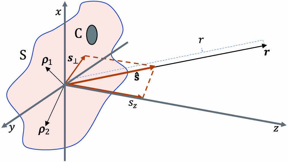
Figure 1.Geometry and notation relating to a quasihomogeneous planar source with an emitting area
In general, the CSD at distance
Our purpose is to model broadband light sources (white LEDs) on the basis of measurable quantities. To this end, we need full information on the source-plane CSD; with that available, we can readily model also the field in the far zone using Eqs. (8)–(10). The source-plane spectral density can be measured straightforwardly by (spectral) imaging, and this allows us to determine the complex degree of angular spectral coherence using Eq. (10). On the other hand, the spectral distribution of the radiant intensity
By Fourier inversion of Eq. (6) and keeping in mind that only the low-frequency (non-evanescent) part of the radiation is observable in the far zone, we have
3. ELEMENTARY-FIELD REPRESENTATION
It is well known that the CSD of any Schell-model field at frequency
Considering a single (fully coherent) elementary field
Let us consider, as an example, well-known cosine-power distributions for radiation from quasihomogeneous sources [6] by writing the radiant intensity in the form
To determine the spectral degree of spatial coherence and the functional form of the elementary field, we insert Eq. (24) into Eq. (16) and Eq. (23), respectively. The integrals involving the Bessel function can be evaluated with the formulas [13]
It is immediately seen that the forms of
Expressions for the Complex Degrees of Coherence and Elementary-Field Distributions for Selected Sources with Radiant Intensities Following the cosp
| 0 | |
| 1 | |
| 2 | |
| 3 | |
| −2 | |
| 0 | |
| 2 | |
| 4 |
Figure 2 illustrates the spatial distributions of
![]()
Figure 2.Plots of the complex degree of coherence for sources with different values of
4. COHERENCE OF SECONDARY SOURCES
Imaging systems with specified NAs are frequently used to generate secondary light sources. In numerous instances, such a secondary source is assumed to be incoherent, though this is always an idealization. The model developed in this paper allows us to evaluate the spectral coherence properties of secondary white-light sources by means of the standard theory of image formation in an aplanatic system [16], illustrated in Fig. 3 in a scalar form.
![]()
Figure 3.Aplanatic image formation in a system with object and image planes
To model the coherence of secondary sources, we employ the same process as in solving the inverse-source problem above. However, we limit the upper integration in Eqs. (16) and (23) only over the collection NA instead of the entire low-frequency part of the angular spectrum. Considering the field in the image space, we then have expressions
According to the sine condition, satisfied by any aplanatic system,
Figure 4 illustrates the distributions of
![]()
Figure 4.Effect of the finite numerical aperture of the imaging system in the elementary-field spread function for (a) Lambertian primary sources with
In general, the effect of reducing the NA leads to widening of the scales of both the effective degree of coherence and the effective elementary field. This effect is, for the degree of coherence, well known in the standard theory of incoherent imaging [4]. Because of the intimate relation between the CSD and the associated elementary field, expressed in Eq. (17), the scale of the latter follows the same trend. It is seen that the distributions of EFS for Lambertian and isotropically radiating primary sources are narrower than those for incoherent sources, and the same applies to the associated degrees of coherence. However, this narrowing happens at the expense of increased sidelobe level. The effect becomes less significant when the NA is reduced, since then only a central region of the low-frequency part of the field is collected and contributes to the EFS function.
5. RELATION TO WOLF’S SCALING LAW
The normalized spectrum
Considering the elementary-field representation of primary sources and assuming a separable distribution of the radiant intensity, it follows from Eq. (23) that
6. COHERENCE OF WHITE LEDS
Our experimental setup for measuring the spectral coherence properties of real white LEDs is shown in Fig. 5. To measure these properties over the full low-frequency region, we place the LED on a rotation stage and any detector D on a fixed spatial position. Three types of measurements have been performed.
![]()
Figure 5.Goniometric experimental setup used for the measurements, with the white LED mounted on a rotation stage R, and a detector D in a fixed position. Polar plots of Lambertian (
![]()
Figure 6.Schematic of the detector setup used for far-field spectral coherence measurement. The solid red line shows the principle ray. BS, beam splitter; LM, corner mirror; G, grating of 300 lines/mm; L, cylindrical lens of focal length
Moderate spectral (and angular) resolution is needed in radiant-intensity measurements. However, the source-plane intensity distribution depends only weakly on wavelength, which justifies the use of bandpass filters in these measurements. In the setup of Fig. 6, spectral interference fringes formed at CAM in the direction perpendicular to the plane of the paper allow the measurement of
We consider in detail the results for two representative white LEDs. The first (ProLight Opto, PM2E-3LWS-SD cool white) is nearly Lambertian because the dome that encloses the active LED structure is more or less hemispherical. We will refer this as a “Lambertian” LED. The second LED (SLOAN, L5-W602-PQBC, cool white) has a collimating dome, and it therefore has a more directional radiant intensity pattern.
Figures 7(a) and 7(b) show the directly measured far-field spectra as a function of the diffraction angle for the Lambertian and directional LEDs in arbitrary units, respectively. Both spectra consist of a blue peak due to the primary LED and a wider yellow peak due to fluorescence, which are at approximately the same positions on the wavelength scale for both LEDs. Looking along the
![]()
Figure 7.Measured radiant intensities as a function of wavelength and
Figures 7(c) and 7(d) show the normalized spectra
With all this being said, it is interesting to consider the case of low- or high-pass filtering of the spectrum. If we filter out the blue part at
Finally, Figs. 7(e) and 7(f) show the source-plane distributions of the absolute values of the complex degree of coherence
Measured source-plane distributions of the spectral density across the Lambertian LED through different narrowband filters are shown in the top row of Fig. 8. These measurements were done by adjusting the imaging system to produce the most compact image obtainable through the aberrated dome; hence, the results should be considered as images of a virtual planar source. Although the true emitting area of the blue primary LED is probably square shaped, we see blurring due to the 3D structure of the phosphor region and aberrations of the dome. For the directional LED, the results are qualitatively similar (though even more blurred), but the effective source size is larger due to the collimation effect of the dome. As expected, the results show only weak frequency dependence. However, the effective size of the virtual source nevertheless increases with the wavelength.
![]()
Figure 8.Top row (a), (c), (e), (g): measured source-plane intensity distributions through spectral filters with central transmission wavelengths at 488, 515, 532, and 633 nm, respectively. Second row (b), (d), (f), (h): numerically calculated absolute values of the complex degree of angular spectral coherence. Third row (i)–(l): cross sections of measured interference patterns (blue) and their envelopes (red) in the far field. Bottom row: comparison of numerically calculated (m) and measured (n) angular spectral coherence.
The second row in Fig. 8 shows the absolute values of the far-field complex degree of spectral coherence
The final two rows of Fig. 8 illustrate the results more quantitatively, by means of cross sections. The third row shows the (normalized) interference patterns recorded with the wavefront-folding interferometer in Fig. 6, and their envelopes. Indeed, the wavelength dependence of these results is weak. In Figs. 8(m) and 8(n), we plot collectively the cross-sectional profiles
7. ANALYTICAL COHERENCE MODELS
We proceed to develop analytical models for the spectral distribution of spatial coherence properties of white LEDs, based on measurements of the type described in the previous section. In view of Figs. 7(c) and 7(d), we have two distinct spectral peaks in the normalized far-field spectra, which suggests that the spectral model should be expressed as a sum of blue (B) and yellow (Y) contributions. On the other hand, in view of Figs. 7(a) and 7(b), we see that the angular distribution of
Motivated by the approach in Ref. [6], we express the functions
It may be worth stressing at this point that the model given by Eq. (44) no longer assumes the separability of the radiant intensity in angular and spectral contributions in the sense of Eq. (24). It now remains to find analytical expressions for the spectral contributions
The model parameters obtained for the angular distributions of the radiant intensity, given by
Model Parameters for the Angular Distribution of Radiant Intensity of the Lambertian and Directional LEDs
| Model [Eq. ( | ||||
| Lambertian | 1.65 | 1.20 | 1.97 | 0.77 |
| Directional | 1.45 | 0.77 | 49.9 | 57.1 |
| Lambertian | 1.46 | 1.17 | 1.44 | 0.94 |
| Directional | 1.47 | 0.67 | 49.5 | 59.5 |
Sign up for Photonics Research TOC. Get the latest issue of Photonics Research delivered right to you!Sign up now
The parameters obtained by least-squares fitting for
Model Parameters for the Spectral Distribution of Lambertian and Directional LEDs
| Model [Eq. ( | ΩB | ΩY | ||
| Lambertian | 4.17 | 0.21 | 3.37 | 0.23 |
| Directional | 4.17 | 0.14 | 3.35 | 0.21 |
| 0.23 | 0.23 | |||
| 0.078 | 0.069 | |||
| −0.15 | −0.16 | |||
| 0.18 | 0.15 | |||
| 3.68 | 3.68 | |||
| 2.07 | 2.07 | |||
All angular frequencies are in units rad/fs.
Figure 9 shows a quantitative comparison of certain cross sections of experimentally measured radiant intensities and those given by the analytic models. In the top row, we illustrate the angular distributions of radiant intensity, and in the bottom row, the axial spectral distributions. The axial spectra are indeed represented well, especially by Eq. (52). The angular distributions match well for the Lambertian LED, and also for the directional LED in the yellow region. In the blue region, there is some mismatch, indicating that a single cosine power does not represent the radiant intensity accurately. The match could be improved by using a second cosine term as in Eq. (5-3-54) of Ref. [6].
![]()
Figure 9.Top row: distributions of
Finally, in Fig. 10, we present a comparison between the numerically calculated distribution of the source-plane complex degree of coherence, and the same calculated using Eq. (52), for the Lambertian LED. The numerically calculated absolute value and phase of the complex degree of coherence are shown in (a) and (b), and the model results given by Eq. (52) are illustrated in (c) and (d). We find that the prediction of the spectral degree of spatial coherence by the model is excellent. Moreover, the width of spatial coherence at the source plane decreases as the optical angular frequency increases except around
![]()
Figure 10.Comparison between the numerically calculated distribution of the source-plane complex degree of coherence and from analytical model [Eq. (
8. DISCUSSION AND CONCLUSION
Most of the work on spatially partially coherent fields, and on radiation that they emit, has over the past decades been mainly concentrated on quasimonochromatic sources and fields. While real sources of thermal or quasi-thermal light were of primary concern in the past, the advent of lasers changed the situation rather dramatically: it was no longer necessary to worry about the low brightness of previously available sources. Moreover, partial spatial coherence could be introduced artificially, e.g., by passing a single-mode laser beam through a rotating diffuser. With the advent of bright LEDs, we are now again in a new situation, having a class of bright sources available that are inherently partially spatially coherent and, moreover, an integral part of present-day life. However, these sources are broadband, not quasimonochromatic.
In our opinion, white LEDs should not be considered merely as lighting devices but be taken under consideration as light sources in near-future (theoretical as well as experimental) scientific studies on coherence properties of light. Thorough understanding of the spatial coherence of white LEDs becomes vital at this stage. In this paper, we have taken some steps in this direction by presenting simple analytical models for their spectral coherence. Our formulation could be readily extended in several ways, such as increasing the number of cosine terms in Eq. (42) in analogy with Eq. (5-3-54) of Ref. [6]. One could also introduce better fits into the spectral distributions of the blue and yellow parts, for instance, by replacing the Gaussian profile assumed here with more sophisticated asymmetric profiles or adding extra Gaussian profiles centered at different frequencies and then fitting them in experimental results. However, the spectral model in Eq. (52) is sufficient for most purposes.
To conclude, we started from theoretical considerations based on the inverse-source problems in partially coherent optics, taking the field to have a finite bandwidth instead of being quasimonochromatic. With the aid of measurements of real white LEDs, we developed models that are sufficiently simple to be used as a starting point of theoretical or experimental analysis of many phenomena or systems related to partially coherent light. Yet the models are sufficiently accurate to reflect the properties of real white LEDs. One of our key findings is that the LED with a near-Lambertian frequency-integrated radiant intensity has a super-Lambertian (
Finally, the identification of the sub-Lambertian radiation, which in our opinion originates from the volume nature of the fluorescence radiation from the true 3D physical source, could benefit microscopy. The resolution in microscopy is limited by the coherence area of the illumination [4], which is below that of the conventional limit (for critical and Köhler illumination) already for the Lambertian source. The reduction is enhanced further for sub-Lambertian sources, though only at the expense of increased sidelobe level.
References
[4] M. Born, E. Wolf. Principles of Optics(1999).
[5] H. P. Baltes, J. Geist, A. Walther. Radiometry and coherence. Inverse Source Problems, 119-154(1978).
[6] L. Mandel, E. Wolf. Coherence and Quantum Optics(1995).
[13] I. S. Gradshteyn, I. M. Ryshik. Table of Integrals, Series, and Products, 687(2014).
[15] J. Turunen, A. T. Friberg. Propagation-invariant optical fields. Progress in Optics, 54, 1-88(2009).
[16] L. Novotny, B. Hecht. Principles of Nano-Optics(2012).


Set citation alerts for the article
Please enter your email address

© Copyright 2018-2021 | Chinese Laser Press. All Rights Reserved 沪ICP备15018463号-20