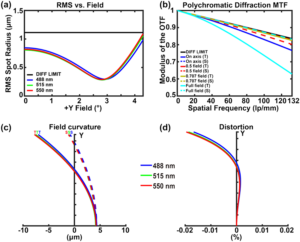
Fig. 1. Relay system performance analysis. (a) RMS spot radius as a function of field (incident degree). The black line indicates the diffraction limit. (b) MTF plot in image space. (c) and (d) Predicted field curvature and distortion plots in image space, respectively. T, tangential plane; S, sagittal plane.

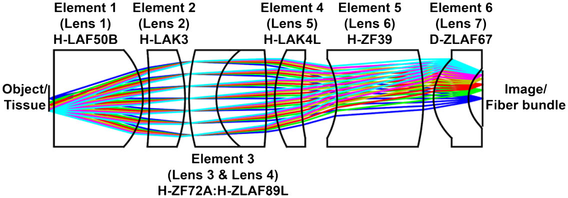
Fig. 2. Schematic diagram of the large-FOV miniature objective lens.

Fig. 3. Spot diagrams with diffraction-limited Airy disks for six radial image positions. The Airy disk spot radius is 1.272 μm.

Fig. 4. (a) Polychromatic diffraction MTFs plot and (b) chromatic focal shift in fiber bundle space of the large-FOV miniature objective lens. DIFF LIMIT, diffraction limit; T, tangential plane; S, sagittal plane.

Fig. 5. Predicted (a) field curvature and (b) distortion plots in fiber bundle space of the large-FOV miniature objective lens.

Fig. 6. Photographs of the large-FOV miniature objective lens and testing results. (a) Large-FOV miniature objective lens placed next to a Chinese 50-cent coin for perspective. (b) Testing results of resolution. (c) Calculated MTF curves from (b).

Fig. 7. (a) Packaged large-FOV pCM system with a fiber-optic probe. Measurement results of the (b) FOV and (c) lateral resolution with line profile analysis result for the vertical features in Group 8 Element 1. The red arrow in (c) points to the smallest resolved details. The scale bars in (b) and the enlarged red box in (c) are 50 and 20 μm, respectively.

Fig. 8. Resolution measurement results. (a)–(c) Resolution measured in three fields of orientation 1. (d)–(f) Resolution measured in three fields of orientation 2. (g)–(i) Resolution measured in three fields of orientation 3. (j)–(l) Resolution measured in three fields of orientation 4. (m)–(o) Line profile analysis results for the vertical features in Group 8 Element 1 in three fields of orientation 4. Red arrows indicate different orientations and point to the smallest resolved details. All positions can clearly distinguish the Group 8 Element 1 bars, corresponding to a bar width of 1.95 μm. Scale bar: 50 μm.

Fig. 9. Comparison of healthy gastric tissue images using a large-FOV pCM and conventional pCM. (a) Image of healthy stomach using the large-FOV pCM. (b) Corresponding histologic specimens. (c) Image of healthy gastric tissues using the conventional pCM. (d) Statistics regarding the number of gastric pits observed in the two pCMs. The t-test was applied (****p<0.0001). Red arrows, superficial epithelial cells; blue arrows, gastric pits. Scale bars: 50 μm.

Fig. 10. Healthy colon tissue images obtained using large-FOV and conventional pCMs. (a) Image of healthy colon obtained using the large-FOV pCM. (b) Corresponding histologic specimens. (c) Image of healthy colon obtained using the conventional pCM. (d) Statistics regarding the number of colon crypts observed in the two pCMs. The t-test was applied (****p<0.0001). Red arrows, columnar epithelial cells; blue arrows, goblet cells; green arrowheads, opening of the crypts. Scale bars: 50 μm.

Fig. 11. Images of healthy and ulcerated gastric tissues. (a) Image of healthy gastric tissue. The mucosa shows regularly distributed superficial epithelial cells (red arrow) and gastric pits (blue arrow) and is free of fluorescein sodium leakage. (b) Image of gastric ulcer. Epithelial cells surrounded by a white circle (red arrow) of normal size and morphology are visible. The gastric ulcer shows distorted gastric pits with dilated openings (blue arrow) and destroyed epithelium with fluorescein sodium leakage (yellow arrow). (c) Histopathological analysis of gastric ulcer tissues. In (c), the red arrow shows epithelial cells, the blue arrow shows gastric pits, and the green arrow shows hemorrhage. Scale bars: 50 μm.

Fig. 12. Images of the colon tissue. (a) A mosaic image of healthy colon tissues includes seven frames obtained using the large-FOV pCM. (b) Enlarged details of the red rectangle in (a). (c) A mosaic image of ulcerative colitis tissues includes eight frames obtained using the large-FOV pCM. (d) Enlarged details of the blue rectangle in (c). (e) A mosaic image of the same ulcerative colitis tissues includes 12 frames obtained using the conventional pCM. (f) Corresponding histological specimens of ulcerative colitis tissues. (g) Crypt numbers observed in the three mosaic images. Red arrows, columnar epithelial cells; blue arrows, goblet cells; yellow arrows, fluorescein sodium leakage; green arrows, crypt fusion; white arrows, dilated openings. In (a), (c), (e), and (f) the scale bars are 100 μm. In (b) and (d), the scale bars are 50 μm.

Fig. 13. Relay system layout. The blue arrow indicates the coupling objective lens. The red arrow indicates the image surface at which the aberrations were calculated. The total optical length of the relay lens system is 608.918 mm.

Fig. 14. (a) RMS wavefront error as a function of field with respect to the diffraction-limited value. (b) RMS spot radius as a function of field with respect to the single fiber radius.

Fig. 15. Schematic of the large-FOV pCM system. DM, dichroic mirrors; OD, outer diameter; FL, focal length; NA, numerical aperture; L, length of the fiber bundle; d, distance between the neighboring fiber cores.

Table 1. Mosaic Image Data