Single-scan polarization-resolved degenerate four-wave mixing spectroscopy using a vector optical field

Jiaqi Yuan; Xuemei Cheng; Xing Wang; Tengfei Jiao; Zhaoyu Ren

doi:10.1364/PRJ.423799

Abstract

We report on a new method to achieve the single-scan polarization-resolved degenerate four-wave mixing (DFWM) spectroscopy in a Rb atomic medium using a vector optical field, in which two pump beams are kept linearly polarized and a vector beam is employed as the probe beam. As the polarization and intensity of the DFWM signal are closely dependent on the polarization state of the probe beam, a vector probe beam with space-variant states of polarization is able to generate a DFWM signal with space-variant states of polarization and intensity across the DFWM image. Accordingly, the polarization-resolved spectra can be retrieved from a single DFWM image. To the best of our knowledge, this is the first time that the single-scan polarization-resolved spectrum detection has been realized experimentally with a vector beam. This work provides a simple but efficient single-scan polarization-resolved spectroscopic method, which would be of great utility for the samples of poor light stability and fast optical processes.

1. INTRODUCTION

Nonlinear optics plays an important role in modern science and technology [1 –3]. Four-wave mixing (FWM) is an important third-order nonlinear optical process, owning wide applications in many areas. Besides its significance in generating quantum-correlated beams and phase-conjugated beams [4,5], FWM also serves as an effective spectroscopic method of many advantages. Resulting from a fully resonant process, FWM spectroscopy has high signal-to-noise ratios (SNRs), which allows for the sensitive and selective detection of stable and transient molecules [6]. Furthermore, the FWM signal is coherent and therefore the entire signal can be collected (rather than a small fraction as compared to an incoherent process like Raman scattering or laser-induced fluorescence) [7]. In addition, the FWM signal is separated from the input beams in direction and thus free from parasitic background fluorescence under proper phase-matching conditions, which further enhances the SNR and makes remote probing possible [8]. So far, FWM spectroscopy has been successfully applied in transient species analysis during combustion [9], isotope ratio measurement [10], and investigation of the energetic structure or dynamic processes of molecules [11,12].

As FWM in many systems is polarization sensitive, polarization-resolved FWM spectral technology is of particular importance. For example, it can be used to reveal the structure and molecular orientation in complex systems [13,14], such as proteins, lipids, and cell membranes. Munhoz and Rigneault have shown that polarization-resolved FWM is a powerful technique for retrieving the even orders of symmetry up to the fourth order in thick collagenous tissues [15]. Polarization-resolved FWM can also be used to determine the third-order nonlinear optical tensor of various media, including transient systems, such as ionized atmospheric air [16] and plasmon excitation on flat graphene [17]. In addition, polarization-resolved FWM is a significant tool for studying the complicated dynamics of nonlinear optical processes, e.g, interwell carrier dynamics [18], ultrafast dynamics in single gold nanoparticles [19], excitonic dephasing [20].

The polarization-resolved FWM is commonly realized by scanning the polarization of incident beams and detecting the signals in sequence. However, such shot-to-shot methods might cause irreversible damage to the samples, and therefore it is not suitable for those samples with poor light stability [15]. Moreover, the modulation speed of the commonly used polarization modulator, such as the electro-optic modulator (EOM), is less than 100 MHz, and thus the transient processes occurring in 10 ns cannot be resolved by shot-to-shot polarization-resolved FWM. Previously, Shalit and Prior proposed an idea of single-scan polarization-resolved FWM where a single incident pulse is spatially encoded with various states of polarization for FWM generation [21]. They also designed an experimental scheme in which an echelon mirror is used to split a pulse into multiple sub-pulses, and then a set of spatial light modulators are employed to modulate the sub-pulses into various states of polarization. However, no results have been reported based on such an experimental geometry.

Sign up for Photonics Research TOC. Get the latest issue of Photonics Research delivered right to you！Sign up now

The vector fields are inherently characterized by space-variant states of polarization. In recent years, vector fields have attracted great attention and have had wide applications in optical micro-manipulation and trapping [22], high-resolution imaging [23], quantum communication [24], etc. Nonuniform spatial polarization provides researchers with one more degree of freedom in studying and utilizing the light–matter interaction. For example, based on the nonlinear interaction of the vector beam and the media, people are able to realize spatial filtering of the vector probe beam based on saturated absorption [25], generate specially correlated radially polarized beams [26], generate the dressed vortex FWM signal and study the modulation effect of the vortex beam on the signal [27], manipulate and select the spatial polarization distribution of a beam [28], etc. We previously realized multi-wave mixing (MWM) generation using a single vector beam, in which we split a vector beam into multiple parts by a polarizer and then focused the multiple parts into the sample to realize MWM [29].

In this work, we propose a new scheme of the single-scan polarization-resolved degenerate four-wave mixing (DFWM) based on a vector field and demonstrate its feasibility with the atomic Rb vapor sample. In the experimental configuration, two pump beams are kept linearly polarized and a vector beam is employed as the probe beam. Utilizing the space-variant polarization of the probe beam, the measurement of the single-scan polarization-resolved spectrum is easily achieved, since the complicated polarization encoded process is avoided. This work not only provides a simple but efficient single-scan polarization-resolved DFWM method, but also provides a method for designing other single-scan polarization-resolved spectral or imaging methods, which would be of significance for low light stability and fast optical processes.

2. EXPERIMENTAL SETUP

Figure 1(a) shows the scheme of our experimental setup. The output from a wavelength tunable continuous-wave (CW) Ti: sapphire laser (Spectra-Physics, Matisse TR) with a spectral linewidth of $\sim 20 MHz$ and a beam size of $\sim 2 mm$ is split into two beams by a polarization beam splitter (PBS1). The transmission through PBS1 is further split into two beams (denoted as $E_{2}$ and $E_{3}$ , pump beams) by PBS2. The reflection from the PBS1 is converted into a vector beam field using a vortex retarder (VR, LBTEK, VR1-780) (denoted as $E_{1}$ , probe beam). The VR is an optical component capable of generating a vector-polarized beam and a vortex beam, which can be realized by using a liquid crystal and a liquid crystal polymer combined with advanced optical phase-matching technology [30]. The VR used in this work is made of liquid crystal polymers, in which the direction of the fast axis varies continuously around the center of the circle.

(a) Scheme of the experimental setup. Ti:S, Ti:sapphire laser; VR, vortex retarder; HR, high reflection mirror; PBS, polarization beam splitter; and HWP, half-wave plate. (b) Phase-matching configuration of forward four-wave mixing geometry. (c) The related energy level structures of Rb87.

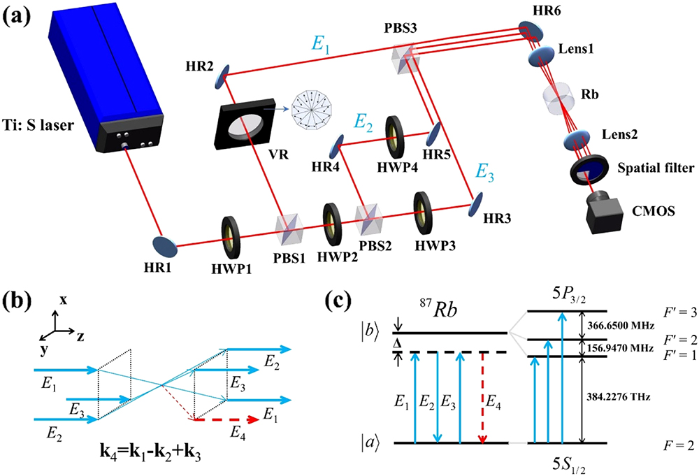
Figure 1.(a) Scheme of the experimental setup. Ti:S, Ti:sapphire laser; VR, vortex retarder; HR, high reflection mirror; PBS, polarization beam splitter; and HWP, half-wave plate. (b) Phase-matching configuration of forward four-wave mixing geometry. (c) The related energy level structures of ${}^{87}{Rb}$ .

The beams $E_{2}$ and $E_{3}$ are further reflected by PBS3, which means $E_{2}$ and $E_{3}$ are both s-polarized when participating in the DFWM process. The probe beam $E_{1}$ propagates over the PBS3. Then, the three beams ( $E_{1}, E_{2}$ , and $E_{3}$ ) are guided to propagate in parallel and then are focused into the Rb atomic cell through an $f = 400 mm$ lens. The power of each incident beam is set to be $\sim 3 mW$ . The radius of each incident beam at focus is $\sim 312 μm$ . The intensity of the incident beams is estimated to be $\sim 980 mW/ {cm}^{2}$ , and therefore the transition involved in this work is saturated (the saturation intensity for the $| 5 S_{1 / 2} ⟩ \to | 5 P_{3 / 2} ⟩$ of ${}^{87}{Rb}$ is $\sim 2.5 mW/ {cm}^{2}$ [31]). The DFWM signal is generated when the three beams interact with the Rb atoms under the phase-matching condition, as shown in Fig. 1(b). In the Cartesian coordinate frame shown in Fig. 1(b), the laser propagates along the $z$ -axis, the s-polarization is along the $x$ -axis, and the p-polarization is along the $y$ -axis. Thereby, the polarizations of $E_{2}$ and $E_{3}$ are kept along the $x$ -axis, and the polarization of $E_{1}$ is variable in the $x - y$ plane.

The Rb sample cell (15 mm in length and 20 mm in diameter) contains the Rb substrate and can be heated by a heater belt to produce Rb atomic vapor. During the experiments, the temperature of the cell was kept at 338.15 K, and the Rb atomic number density is approximated to be $5 \times 10^{6} {cm}^{- 3}$ or so [31]. The energy states $| 5 S_{1 / 2} ⟩$ and $| 5 P_{3 / 2} ⟩$ in the $D_{2}$ line of ${}^{87}{Rb}$ are involved in this work. The state of $| 5 S_{1 / 2} ⟩$ includes two hyperfine levels $| 5 S_{1 / 2}, F = 1, 2 ⟩$ , and the state of $| 5 P_{3 / 2} ⟩$ includes four hyperfine levels $| 5 P_{3 / 2}, F = 0, 1, 2, 3 ⟩$ . As the $| 5 S_{1 / 2}, F = 2 ⟩$ (denoted as the ground state $| a ⟩$ ) is chosen as the ground state, the excited state should be $| 5 P_{3 / 2}, F = 1, 2, 3 ⟩$ according to the selection rules. Because the three hyperfine levels of $| 5 P_{3 / 2}, F = 1, 2, 3 ⟩$ cannot be resolved in the DFWM spectrum due to Doppler broadening, we plot them as one line (denoted as the excited state $| b ⟩$ ) in the energy level diagram shown in Fig. 1(c). The laser wavelength is fixed at 780.2459 nm, resonant to the transition of ${}^{87}{Rb} | 5 S_{1 / 2}, F = 2 ⟩ \to | 5 P_{3 / 2}, F^{'} = 1, 2, 3 ⟩$ .

As for the detecting part, the images of the DFWM signal are captured by a CMOS camera. A spatial filter is placed in front of the CMOS camera to filter out the incident beams. A polarization analyzer is inserted before the CMOS camera when we determine the polarization distribution of the signal beam (not shown). The polarization analyzer we used is a Glan prism.

3. THEORETICAL CONSIDERATIONS

The third-order nonlinear polarization is deduced with density-matrix formalism $ρ$ . Based on the perturbation theory [32], the perturbation chains related to the FWM process in a two-level system can be written as (1) $ρ_{aa}^{(0)} \overset{E_{1}}{\to} ρ_{ba}^{(1)} \overset{E_{2}^{*}}{\to} ρ_{aa}^{(2)} \overset{E_{3}}{\to} ρ_{ba}^{(3)}$ and (2) $ρ_{aa}^{(0)} \overset{E_{3}}{\to} ρ_{ba}^{(1)} \overset{E_{2}^{*}}{\to} ρ_{aa}^{(2)} \overset{E_{1}}{\to} ρ_{ba}^{(3)}$ [shown in Fig. 1(c)]. Here $E_{1} = E_{1} (ω_{1}) e^{- i ω_{1} t}$ is the probe beam with the frequency of $ω_{1}$ , and $E_{2} = E_{2} (ω_{2}) e^{- i ω_{2} t}$ and $E_{3} = E_{3} (ω_{3}) e^{- i ω_{3} t}$ are pump beams with the frequencies of $ω_{2}$ and $ω_{3}$ , respectively.

Then, the expression of the third-order density matrix elements [32] can be derived using these chains $ρ_{b a 1}^{(3)} = \frac{1}{ℏ^{3}} \frac{[μ_{b a} \cdot E_{3} (ω_{3})] [μ_{a b} \cdot E_{2}^{*} (ω_{2})] [μ_{b a} \cdot E_{1} (ω_{1})] e^{- i (ω_{1} - ω_{2} + ω_{3}) t}}{[(ω_{b a} - ω_{1} + ω_{2} - ω_{3}) - i / T_{2}] [(ω_{2} - ω_{1}) + i / T_{1}] [(ω_{ba} - ω_{1}) - i / T_{2}]},$ (1) $ρ_{b a 2}^{(3)} = \frac{1}{ℏ^{3}} \frac{[μ_{b a} \cdot E_{1} (ω_{1})] [μ_{a b} \cdot E_{2}^{*} (ω_{2})] [μ_{b a} \cdot E_{3} (ω_{3})] e^{- i (ω_{3} - ω_{2} + ω_{1}) t}}{[(ω_{b a} - ω_{3} + ω_{2} - ω_{1}) - i / T_{2}] [(ω_{2} - ω_{3}) + i / T_{1}] [(ω_{ba} - ω_{3}) - i / T_{2}]},$ (2)where $T_{1} = 1 / Γ_{b a}$ is the lifetime of the excited state, and $T_{2} = 1 / γ_{b a}$ is the relaxation time of the transition of the dipole moment. The induced third-order polarization [32] is obtained by $P^{(3)} = N μ_{a b} ρ_{b a}^{(3)} = N μ_{a b} (ρ_{b a 1}^{(3)} + ρ_{b a 2}^{(3)}),$ (3)where $ρ_{b a}^{(3)} = ρ_{b a 1}^{(3)} + ρ_{b a 2}^{(3)}$ , $N$ is the atom number density, and $μ_{a b}$ is the transition dipole between $| a ⟩$ and $| b ⟩$ .

For DFWM, the frequencies of three incident beams are the same: $ω_{1} = ω_{2} = ω_{3} = ω$ , and therefore the third-order atomic polarization of the DFWM signal [32] is $P_{b a}^{(3)} = \frac{2 N}{ℏ^{3}} \frac{μ_{a b} [μ_{b a} \cdot E_{1} (ω)] [μ_{a b} \cdot E_{2}^{*} (ω)] [μ_{b a} \cdot E_{3} (ω)]}{(Δ + i / T_{2}) (i / T_{1}) (Δ + i / T_{2})} e^{- i ω t},$ (4)where the laser detuning is denoted as $Δ = ω - ω_{b a}$ .

The coupling wave equation under the slowly varying amplitude approximation is $2 i k \frac{\partial E_{p}}{\partial z} - μ_{0} ε_{0} ε_{r} (\frac{\partial^{2} E_{p}}{\partial t^{2}} - 2 i ω \frac{\partial E_{p}}{\partial t}) = μ_{0} (\frac{\partial^{2} P_{p}^{N L}}{\partial t^{2}} - i ω \frac{\partial P_{p}^{N L}}{\partial t} - ω^{2} P_{p}^{N L}) e^{i Δ k z} .$ (5)Then, considering the fact that the light source we used was a continuous-wave laser, we can neglect the terms related to time (the so-called steady-state approximation) and get $2 i k_{p} \frac{\partial E_{p}}{\partial z} = - μ_{0} ω_{p}^{2} P_{p}^{N L} e^{i Δ k z} .$ (6)As for our case, $E_{p}$ is the amplitude of the DFWM signal $E_{4}$ , $P_{p}^{N L}$ is the third-order polarization $P^{(3)}$ , and $Δ k = 0$ under the phase-matching condition. So the coupled-wave equation of the DFWM process can be expressed as $\frac{\partial E_{4}}{\partial z} = \frac{i ω^{2}}{2 ε_{0} c n} P^{(3)},$ (7)where $ε_{0}, c$ , and $n$ are the permittivity of the vacuum, the speed of light, and the refractive index, respectively. With the boundary condition $E_{4} (z = 0) = 0$ , we can get the amplitude of the DFWM signal, $E_{4} (z) = \frac{i ω^{2}}{2 ε_{0} c n} P^{(3)} z .$ (8)It is seen that the generated DFWM amplitude $E_{4}$ is in proportion to the third-order atomic polarization intensity ( $E_{4} \propto P^{(3)}$ ). Hence, the intensity of the DFWM signal $I_{4}$ can be represented by $| P^{(3)} |^{2}$ . According to the expression of the third-order polarization $P^{(3)}$ in Eq. (4), the efficiency of the DFWM process can be improved by tuning the laser wavelength resonant to the atoms ( $Δ = 0$ ) and increasing the atomic number density $N$ . It is also found that we can improve the efficiency by exciting the DFWM process in the transitions with a larger dipole moment $μ_{a b}$ , which can be realized by varying the polarization of the incident beams.

To clearly describe the interaction between the atom and the polarized beams, we discuss the situations when the polarization state of $E_{1}$ is varied while $E_{2}$ and $E_{3}$ are kept $x$ -polarized. The treatment of the incident beams is that an arbitrarily polarized beam is projected into the $x$ and the $y$ directions to get the $x$ -polarized and the $y$ -polarized components. When interacting with the Rb atoms, the $x$ -polarized component remains linearly polarized, while the $y$ -polarized component is decomposed into equally left-circular ( $σ^{+}$ ) and right-circular ( $σ^{-}$ ) polarized components.

As shown in Fig. 1(c), three transitions $| 5 S_{1 / 2}, F = 2 ⟩ \to | 5 P_{3 / 2}, F^{'} = 1 ⟩$ , $| 5 S_{1 / 2}, F = 2 ⟩ \to | 5 P_{3 / 2}, F^{'} = 2 ⟩$ and $| 5 S_{1 / 2}, F = 2 ⟩ \to | 5 P_{3 / 2}, F^{'} = 3 ⟩$ are used in the DFWM process in this work. We take the transition path from $F = 2$ to $F^{'} = 1$ as an example to illustrate the interaction of the system with the polarized incident beams. Figure 2 shows the allowed transition paths generating a DFWM signal in different polarization configurations from $F = 2$ to $F^{'} = 1$ . To quantitatively estimate the contribution of each of the DFWM processes under various polarization configurations, we calculated the Rabi frequency of every allowed transition according to $Ω = μ_{a b} E / ⏧$ , in which $μ_{a b}$ is the transition dipole moment for the $| a ⟩ \to | b ⟩$ transition, $E$ is the electric field, and $ℏ$ is the reduced Planck constant. The transition dipole moment $μ_{a b}$ varies with different transition paths between hyperfine energy levels, which can be obtained by multiplying the transition dipole moment of $| 5 S_{1 / 2} ⟩$ and $| 5 P_{3 / 2} ⟩$ in the $D_{2}$ line of ${}^{87}{Rb} (\sim 3.584 \times 10^{- 29} C \cdot m)$ with a coefficient for specific hyperfine transition provided by Steck [31]. The Rabi frequency is denoted as $Ω_{j k}^{l}$ , where $j = 1$ , 2, 3, or 4 represents the beams $E_{1}, E_{2}, E_{3}$ , and $E_{4}$ , respectively; $l = π, σ^{+}, σ^{-}$ stands for the polarization state of the beams; and $k = 1$ , 2, or 3 stands for the set of the DFWM process, as indicated in Fig. 2. The allowed transition paths for the cases of $F = 2$ to $F^{'} = 2$ and 3 can be calculated similarly by the transition rule.

Figure 2.Possible transition paths at different polarization configurations from $| 5 S_{1 / 2}, F = 2 ⟩$ to $| 5 P_{3 / 2}, F^{'} = 1 ⟩$ in the $D_{2}$ line of ${}^{87}{Rb}$ when the probe beam is (a) $x$ -polarized, (b) $σ^{+}$ , and (c) $σ^{-}$ . $F$ is the total angular momentum quantum number, and $m_{F}$ is the corresponding projection value. $Ω_{j k}^{l}$ are the corresponding Rabi frequencies of the transitions, which are $Ω_{11}^{π} = Ω_{21}^{π} = Ω_{31}^{π} = Ω_{41}^{π} = Ω_{13}^{π} = Ω_{23}^{π} = Ω_{33}^{π} = Ω_{43}^{π} = Ω_{11}^{σ +} = Ω_{41}^{σ +} = Ω_{13}^{σ -} = Ω_{43}^{σ -} = \sim 146 MHz$ , $Ω_{12}^{π} = Ω_{22}^{π} = Ω_{32}^{π} = Ω_{42}^{π} = \sim 169 MHz$ , $Ω_{12}^{σ +} = Ω_{42}^{σ +} = Ω_{12}^{σ -} = Ω_{42}^{σ -} = \sim 103 MHz$ , and $Ω_{13}^{σ +} = Ω_{43}^{σ +} = Ω_{11}^{σ -} = Ω_{41}^{σ -} = \sim 60 MHz$ .

It is seen from Fig. 2 that the transition paths are different for different polarization states of $E_{1}$ . As the transition dipole moment $μ_{a b}$ varies for different transition paths, the generated DFWM signal varies accordingly. When $E_{2}$ and $E_{3}$ are kept invariant, we can write the third-order atomic polarization of the DFWM according to Eq. (4) to be $P^{(3)} = P_{x}^{(3)} + P_{y}^{(3)} \propto A E_{1 x} + B E_{1 y},$ (9)where $A$ and $B$ are the weighting factors for the $x$ -polarized and the $y$ -polarized components of $E_{1}$ , dependent on the transition paths. Through calculation with the known data of $μ_{a b}$ [31], we get that $A = 0.34$ and $B = 0.19$ considering that all the contributions from the allowed transition paths of $| 5 S_{1 / 2}, F = 2 ⟩ \to | 5 P_{3 / 2}, F^{'} = 1, 2, 3 ⟩$ are considered.

4. RESULTS AND DISCUSSION

To determine the dependence of the DFWM signal on the polarization state of the probe beam $E_{1}$ , we first replace the VR with an HWP to scan the polarization direction of $E_{1}$ and measure the intensity of the DFWM signal under various polarization directions of $E_{1}$ . The DFWM intensity versus the rotation angle of the HWP is plotted in Fig. 3. The power of each incident beam is set to be $\sim 3 mW$ , and the highest DFWM signal is measured to be $\sim 50 μW$ . Therefore, the conversion efficiency of the DFWM process is $\sim 0.6 %$ . It is found that the DFWM intensity is highest at 0°, 90°, and 180° and lowest at 45° and 135°. In our experiments, beam $E_{1}$ is $x$ -polarized at 0°, 90°, and 180° and $y$ -polarized at 45° and 135°. Together with the fact that $E_{2}$ and $E_{3}$ are both kept $x$ -polarized in this work, we can see that the results are in agreement with previous studies where the DFWM signal gets highest when the polarizations of the three incident beams are in parallel and lowest when the polarization of $E_{1}$ is perpendicular to that of $E_{2}$ and $E_{3}$ [16].

Figure 3.Normalized DFWM signal intensity with respect to the rotation angle of the HWP varying the polarization of $E_{1}$ . The pump beams $E_{2}$ and $E_{3}$ are kept $x$ -polarized. The red dots are the experimental data, and the black line is the theoretical curve.

Theoretically, when a linearly polarized beam passes through an HWP, its two projected components are $E_{x} = E_{0} \cos (2 θ)$ and $E_{y} = E_{0} \sin (2 θ)$ , where $θ$ is the rotation angle of the HWP with respect to its main axis. Inserting $E_{x}$ and $E_{y}$ into Eq. (7), we can get the theoretical curve (black line). It is seen that the experimental data agrees well with the theoretical curve, indicating that the polarization dependence of the DFWM can be described by the interaction between the polarized light and the atomic hyperfine energy levels. The offsets in the minimum might be caused by the error in measuring the weak signal.

From the above study, we know that the DFWM signal of the Rb atoms is quite sensitive to the polarization of the probe beam $E_{1}$ when the polarizations of the pump beams $E_{2}$ and $E_{3}$ are kept invariant. In order to get the single-scan polarization-resolved DFWM, we then can convert the beam $E_{1}$ from a linearly polarized beam into a vector beam by the VR and take the vector beam as the probe beam to produce the DFWM signal.

The polarization distribution of the vector optical field can be varied by rotating the fast axis of the VR. The typical radial and angular vector fields generated are shown in Fig. 4(a) I and IV, respectively, in which the arrows stand for the polarization distribution of the fields, which can be determined through an analyzer. Figure 4(a) II, III, V, and VI show the beam images after the analyzer. Then, keeping the pump beams $E_{2}$ and $E_{3}$ $x$ -polarized, we obtain images of the single-scan DFWM signal when $E_{1}$ is the radial and angular vector field, respectively, as shown in Fig. 4(b) VII and VIII. It is clearly seen that the DFWM signal intensity is spatially variable across the images, the shapes of which look like two pairs of “cashews.”

Figure 4.Polarization distribution of the single-scan DFWM signal. (a) Beam images of the vector optical field and its corresponding images after the analyzer. (b) Single-scan DFWM signal image when $E_{1}$ is the vector optical field.

To find the relationship between the space-variant intensity of the DFWM signal and the space-variant polarization of $E_{1}$ , we further determined the polarization distribution across the DFWM signal image using an analyzer. Figures 5(a) and 5(b) show the images of the DFWM signal captured after the analyzer, which are obtained when the probe beam $E_{1}$ is a radial and an angular vector field, respectively. It is seen that the polarization state of the DFWM signal is space-variant with an identical polarization distribution of $E_{1}$ . It is to be understood that in the isotropic medium, the polarization state of the DFWM signal is identical to the probe beam $E_{1}$ when the polarization states of $E_{2}$ and $E_{3}$ are kept the same. Therefore, the $x$ -polarized DFWM signal is the result of the $x$ -polarized parts of $E_{1}$ , and the $y$ -polarized DFWM signal is the result of the $y$ -polarized parts.

Figure 5.DFWM signal images after a polarization analyzer: (a) $E_{1}$ is the radial vector optical field, and (b) $E_{1}$ is the angular vector optical field.

According to Fig. 5, we can denote the polarization distribution of the DFWM signal across the beam image as the arrows show in Figs. 6(a) and 6(c). Then, we can discuss the DFWM signal intensity under various polarization directions. It is observed that the DFWM signal intensity is space-variant across the signal image. The DFWM signal gets highest when $E_{1}$ is $x$ -polarized and lowest when $E_{1}$ is $y$ -polarized. Such results can be well explained by the fact that the DFWM signal intensity is dependent on the polarization state of $E_{1}$ (Fig. 3). When a vector beam with space-variant polarization is employed as the probe beam $E_{1}$ , the DFWM signal intensity becomes space-variant.

Figure 6.Polarization distribution across the DFWM images, and the polarization-resolved spectra retrieved from the single DFWM signal when (a) and (b) $E_{1}$ is the radial vector optical field, and (c) and (d) $E_{1}$ is the angular vector optical field. The black solid lines are the theoretical curves.

In this manner, the polarization-resolved spectra can be retrieved from a single DFWM signal image. As shown in Figs. 6(a) and 6(c), we denoted the vertical direction on the DFWM signal images as 0° and segmented the images radially every 15°. Then, we integrated the intensity along the straight lines. Finally, the integrated intensity was plotted with respect to the angle, and the polarization-resolved spectra were thus obtained [Figs. 6(b) and 6(d)]. It is seen that the DFWM signal attains a maximum at $x$ -polarized and a minimum at $y$ -polarized for both cases ( $E_{1}$ is the radial and angular vector optical field, respectively), which is in good agreement with the theoretical curves, indicating that a single vector beam is able to realize polarization-resolved spectrum detection. The offsets in the minimum might be caused by two aspects. First, there is a larger error in measuring the weak signal. Second, only a spatial part of the $E_{1}$ beam participates in the DFWM process for the single-scan case, which might cause even larger measurement errors.

5. CONCLUSION

In this work, we realized the single-scan polarization-resolved DFWM spectroscopy in the Rb atomic medium based on the space-variant polarization characteristics of the vector beam. In the experimental scheme, a vector beam is employed as the probe beam, and the two pump beams remain linearly polarized. As the polarization and intensity of the DFWM signal are closely dependent on the polarization state of the probe beam when the pump beams are kept invariant, a vector probe beam with space-variant states of polarization is able to generate a DFWM signal with space-variant states of polarization and intensity. Therefore, the polarization and intensity information can be retrieved from the single DFWM signal image. Compared with the traditional shot-to-shot polarization-resolved spectroscopy, the single-scan polarization-resolved spectrum is of particular importance in studying the samples of poor light stability and fast optical processes. In addition, the scheme proposed in this work based on the vector field is simple to use. To the best of our knowledge, this is the first time that single-scan polarization-resolved spectrum detection has been realized based on the vector field. This work not only provides a simple but efficient single-scan polarization-resolved DFWM method but also blazes a path for designing other single-scan polarization-resolved spectral or imaging methods, which would be of special significance for the samples of poor light stability and fast optical processes. In the next step, we will apply the single-scan polarization-resolved DFWM method to studying the micro-structure of the biological samples of poor light stability.

References

[1] A. J. Brown. Spectral curve fitting for automatic hyperspectral data analysis. IEEE Trans. Geosci. Remote Sens., 44, 1601-1608(2006).

[2] A. J. Brown. Equivalence relations and symmetries for laboratory, LIDAR, and planetary Müeller matrix scattering geometries. J. Opt. Soc. Am. A, 31, 2789-2794(2014).

[3] A. J. Brown, T. I. Michaels, S. Byrne, W. Sun, T. N. Titus, A. Colaprete, M. J. Wolff, G. Videen, C. J. Grund. The case for a modern multiwavelength, polarization-sensitive LIDAR in orbit around mars. J. Quant. Spectrosc. Radiat. Transfer, 153, 131-143(2015).

[4] N. Gisin, G. Ribordy, W. Tittel, H. Zbinden. Quantum cryptography. Rev. Mod. Phys., 74, 145-195(2002).

[5] A. E. Bracamonte, P. H. Vaccaro. Dissection of rovibronic band structure by polarization-resolved degenerate four-wave mixing spectroscopy. J. Chem. Phys., 119, 887-901(2003).

[6] Z. Liu, Z. Wang, X. Wang, X. Xu, X. Chen, J. Cheng, X. Li, S. Chen, J. Xin, S. T. C. Wong. Fiber bundle based probe with polarization for coherent anti-Stokes Raman scattering microendoscopy imaging. Proc. SPIE, 8588, 85880F(2013).

[7] A. M. Zheltikov, N. I. Koroteev, A. N. Naumov, V. N. Ochkin, S. Y. Savinov, S. N. Tskhai. Measurement of electric fields in a plasma with the aid of the coherent four-wave mixing polarisation technique. Quantum Electron., 29, 73-76(1999).

[8] Y. Prior. Three-dimensional phase matching in four-wave mixing. Appl. Opt., 19, 1741-1743(1980).

[9] G. Knopp, P. P. Radi, T. Gerber. Dispersed fs-FWM for investigations of low frequency vibrations of transient species in combustion. Chimia, 65, 339-341(2011).

[10] X. Cheng, Z. Ren, J. Wang, Y. Miao, X. Xu, L. Jia, H. Fan, J. Bai. Quantitative measurement of rubidium isotope ratio using forward degenerate four-wave mixing. Spectrochim. Acta B Atom. Spectros., 70, 39-44(2012).

[11] R. E. Compton. Nonlinear optics in non-equilibrium microplasmas(2011).

[12] S. Adachi, Y. Takagi, J. Takeda, K. A. Nelson. Optical sampling four-wave-mixing experiment for exciton relaxation processes. Opt. Commun., 174, 291-298(2000).

[13] S. Ye, S. Ma, F. Wei, H. Li. Intramolecular vibrational coupling in water molecules revealed by compatible multiple nonlinear vibrational spectroscopic measurements. Analyst, 137, 4981-4987(2012).

[14] C. Krafft, B. Dietzek, J. Popp. Raman and CARS microspectroscopy of cells and tissues. Analyst, 134, 1046-1057(2009).

[15] F. Munhoz, H. Rigneault, S. Brasselet. Polarization-resolved four-wave mixing microscopy for structural imaging in thick tissues. J. Opt. Soc. Am. B, 29, 1541-1550(2012).

[16] I. V. Fedotov, P. A. Zhokhov, A. B. Fedotov, A. M. Zheltikov. Probing the ultrafast nonlinear-optical response of ionized atmospheric air by polarization-resolved four-wave mixing. Phys. Rev. A, 80, 015802(2009).

[17] J. Tao, Z. Dong, J. K. W. Yang, Q. J. Wang. Plasmon excitation on flat graphene by s-polarized beams using four-wave mixing. Opt. Express, 23, 7809-7819(2015).

[18] R. Paiella, G. Hunziker, K. J. Vahala, U. Koren. Measurement of the interwell carrier transport lifetime in multiquantum-well optical amplifiers by polarization-resolved four-wave mixing. Appl. Phys. Lett., 69, 4142-4144(1996).

[19] F. Masia, W. Langbein, P. Borri. Polarization-resolved ultrafast dynamics of the complex polarizability in single gold nanoparticles. Phys. Chem. Chem. Phys., 15, 4226-4232(2013).

[20] J. Ishi-Hayase, K. Akahane, N. Yamamoto, M. Kujiraoka, J. Inoue, K. Ema, M. Tsuchiya, M. Sasaki. Coherent dynamics of excitons in a stack of self-assembled InAs quantum dots at 1.5-μm waveband. J. Lumin., 119–120, 318-322(2006).

[21] A. Shalit, Y. Prior. Time resolved polarization dependent single shot four wave mixing. Phys. Chem. Chem. Phys., 14, 13989-13996(2012).

[22] Y. Kozawa, S. Sato. Optical trapping of micrometer-sized dielectric particles by cylindrical vector beams. Opt. Express, 18, 10828-10833(2010).

[23] D. P. Biss, K. S. Youngworth, T. G. Brown. Dark-field imaging with cylindrical-vector beams. Appl. Opt., 45, 470-479(2006).

[24] G. Milione, T. A. Nguyen, J. Leach, D. A. Nolan, R. R. Alfano. Using the nonseparability of vector beams to encode information for optical communication. Opt. Lett., 40, 4887-4890(2015).

[25] J. Wang, X. Yang, Z. Dou, S. Qiu, J. Liu, Y. Chen, M. Cao, H. Chen, D. Wei, K. Müller-Dethlefs, H. Gao, F. Li. Directly extracting the authentic basis of cylindrical vector beams by a pump-probe technique in an atomic vapor. Appl. Phys. Lett., 115, 221101(2019).

[26] Y. Chen, F. Wang, L. Liu, C. Zhao, Y. Cai, O. Korotkova. Generation and propagation of a partially coherent vector beam with special correlation functions. Phys. Rev. A, 89, 013801(2014).

[27] J. Che, P. Zhao, D. Ma, Y. Zhang. Kerr-nonlinearity-modulated dressed vortex four-wave mixing from photonic band gap. Opt. Express, 28, 18343-18350(2020).

[28] J. Wang, X. Yang, Y. Li, Y. Chen, M. Cao, D. Wei, H. Gao, F. Li. Optically spatial information selection with hybridly polarized beam in atomic vapor. Photon. Res., 6, 451-456(2018).

[29] T. Jiao, X. Cheng, Q. Zhang, W. Li, Z. Ren. Multi-wave mixing using a single vector optical field. Appl. Phys. Lett., 115, 201104(2019).

[30] S. C. McEldowney, D. M. Shemo, R. A. Chipman. Vortex retarders produced from photo-aligned liquid crystal polymers. Opt. Express, 16, 7295-7308(2008).

[31] D. A. Steck. Rubidium 87 D line data(2021).

[32] R. W. Boyd. Nonlinear Optics(2002).