Hyperbolic media feature extreme optical anisotropy where the component of its permittivity tensor can have different signs, which is widely studied spanning from (known as) metamaterials [1–5] to natural optical crystals [6–12]. Those properties will allow the unbounded hyperbolic dispersions with large momentum of waves, and, hence, the high confinement of light at the nanoscale for enhanced light–matter interactions. As a result, hyperbolic metamaterials [4,5], artificial materials made of metal-dielectric multilayers or plasmonic nanowire arrays, are exploited for numerous applications including negative refraction [2,4,5], subwavelength imaging [1,13,14], and enhanced spontaneous emission [15,16]. However, the substantial plasmonic losses are inevitable. More recently, the hyperbolic response is found in bulky crystals and thin van der Waals (vdW) films, such as hexagonal boron nitride (hBN) [6–8] and α-phase molybdenum trioxide (α–MoO3) [9–12] due to their strong excitation of optical phonons, forming hyperbolic phonon polaritons (PhPs). This kind of hyperbolic response, in principle, is immune from Ohmic loss as a result of the absence of electron–electron scattering and offers tremendous opportunities of nanoscale manipulation of light.

For further controls, one can make the structure of natural crystals. For instance, the structured array of deeply subwavelength hBN gratings [6,7] can allow the in-plane hyperbolic dispersions, facilitating directional propagations of otherwise isotropic polaritons at the interface. Flexible switching of those directions as well as driving hyperbolic to elliptic topological transition can be realized [17,18] using the twisted bilayer configurations. Moreover, the α–MoO3 nanocavities for predescribed field patterns and prolonged lifetime are observed in tailoring the orientation of geometric boundaries [19]. Applications of focusing, wavefront engineering, and electrically dynamical modulation of polaritons are also explored [20–23]. In general, those cases show that structuring anisotropic media can supply even more powers for extreme and exotic light manipulations, thus, in this paper we provided a generic and systematic approach of such structuring deriving from transformation optics (TO) theory for the on-demand designer polaritonics.

TO [24–26] applies spatial coordinate transformations to design spatially varying and anisotropic material composites based on the form invariance of Maxwell’s equations, enabling various fascinating metaphotonic applications, such as invisibility cloaks [27], field rotators [28], cosmic string simulators [29], and mimicked Hawking radiation [30]. However, spatial-transformation-based TO theory has not been well constructed for hyperbolic media because the spatial metric signature experiences a transition from (+,+) to (−,+), which introduces the “pseudotime coordinate,” causing the effect in similar to a space–time exchange [31,32]. A recent work [33] introduces two-dimensional (2D) Clifford algebra to build a theory of hyperbolic conformal TO, but it requires a coordinate weight ratio of space geometry to be 1, which is isotropic to some extent, limiting the material realizability in experiments.

Here, we propose a new Pythagorean theorem in an anisotropic system and build up an anisotropic Fermat’s principle which provides guidelines for polaritons and nanoscale extreme light manipulation via reshaping the space geometry to hyperbolic. We apply this theory to the absolute instruments [34–37], and specifically, we demonstrate the Luneburg lens (LL) for intrinsic collimation and Maxwell’s fish-eye lens (MFL) for interface focusing of hyperbolic PhPs in α–MoO3 layers. Since our theory requires on-site and local modulation of polaritonic characteristics, we show that the simple spatial modulation of thickness of the biaxial α–MoO3 would be enough to implement the proposed anisotropic Fermat’s principle within reasonable experimental efforts in the future [38,39].

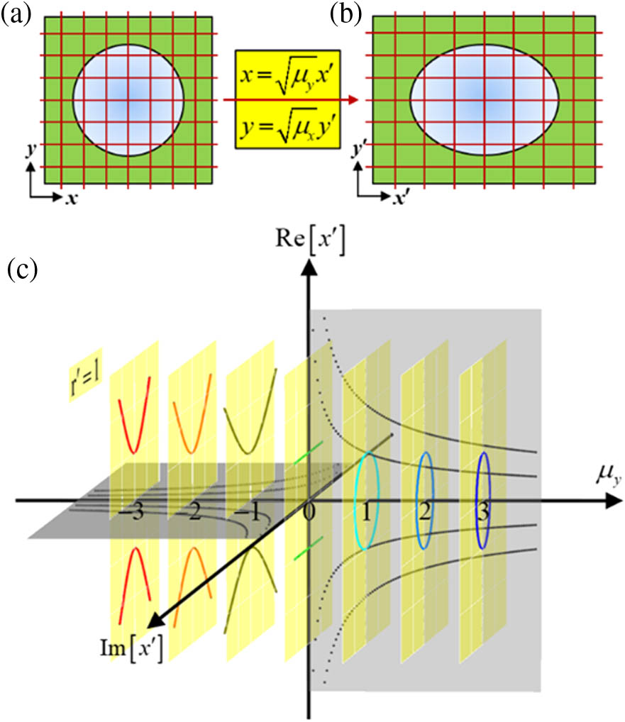
We first discuss our approach towards the TO theory for hyperbolic media. In the following and unless otherwise specified, without loss of generality, we focus on the 2D transverse magnetic (TM) polarization, which is usually much more confined. Assume a space filled with the following material: ε=μ=[10001000n2(x,y)],(1)where the z component of the permittivity and permeability follows the profile n(x,y) with respect to Cartesian coordinates x and y depicted as the red square grids as shown in Fig. 1(a). We here consider a mapping that can afford the transformation towards an anisotropic space, defined as x=μyx′,y=μxy′,(2)where μx and μy are real constants that control the deformation of coordinates. According to the TO recipe [24–26], we can easily obtain material parameters in the (x′,y′) coordinate, shown schematically as the red rectangular grids in Fig. 1(b) from Eq. (1), written as ε′=μ′=[μxμy000μyμx000μxμyn′2(μyx′,μxy′)].(3)

From this equation, we know that εz′=n′2μxμy, μx′=μxμy, and μy′=μyμx for TM polarization. The physical space after the mapping of Eq. (2) can be expressed by a complex number, w′=μyx′+iμxy′.(4)

The use of a complex number has geometrical significance: the modulus |w′|=w′*·w′ gives a generalized radial coordinate, r′=μyx′2+μxy′2,(5)which obeys a new Pythagorean theorem. Euler’s formula form of the complex number w′=r′eiθ′=r′cosθ′+ir′sinθ′ results in cosθ′=μyx′μyx′2+μxy′2 and sinθ′=μxy′μyx′2+μxy′2.

Obviously, the constructed anisotropic space depends on the values of μx and μy. The new space can be freely shaped into an elliptic geometry if μx>0,μy>0. However, it is not able to obtain a hyperbolic medium from Eq. (3) as the material parameters are all in the form of square roots, which cannot give negative values. Besides, the complex number of Eq. (4) would lose its meaning if μxμy<0. This weird phenomenon is demonstrated in Fig. 1(c). For instance, setting μx=1 (a mapping where the y-axis coordinate will not change), the relationship of the x-axis coordinate versus μy is plotted in Fig. 1(c). When the value of μy varies from positive to negative, the transformation mappings of x=μyx′ (illustrated as black stipple lines with x being 2, 1, −1,−2, respectively) will jump from the Re(x′)−μy plane to the Im(x′)−μy plane. This imaginary coordinate actually changes the original space geometry where the conventional TO is defined. A recent work [33] defined a conformal ultrahyperbolic geometry using 2D Clifford algebra. Nevertheless, the weight ratio of coordinates is restricted as 1, i.e., the conic angle of asymptotes is always 90°, this isotropic geometry is quite confined, and the corresponding materials are not easy to achieve in experiments.

Next, we show that the mapping of Eq. (2) can be used to define a more general geometry, which accommodates both hyperbolic and elliptic cases, and establish an anisotropic Fermat’s principle theory, which is easier for further implementation.

From Eq. (2), the line element in the anisotropic space can be defined as ds′2=n′2dl′2=n′2(μydx′2+μxdy′2)=εz′μy′dx′2+εz′μx′dy′2,(6)where dl′=μydx′2+μxdy′2 is the infinitesimal increment of the anisotropic geometrical path length, consistent with the generalized radial coordinate of Eq. (5). This generalized system actually conforms to an anisotropic Fermat’s principle. In addition, we can find a perfect analogy of this anisotropic Fermat’s principle in mechanics based on the optical-mechanical analogy theory [37,40] (see Appendix A). The trajectory of the particle with unit mass, total energy E, and potential U in mechanics is the same as the trajectory of light rays in the refractive index n(r′), n(r′)=2(E−U),(7)where it is noted that the radial coordinate r′ of n(r′) should be the generalized one, that is, Eq. (5) in this anisotropic system.

Thus, from Eq. (6), we can rewrite the material parameters of the anisotropic space as ε′=μ′=[μx000μy000n′2(r′)],(8)where εz′=n′2,μx′=μx, and μy′=μy for TM polarization. The refractive index n′=n′(r′) is a function of Eq. (5), and the factors μx and μy are exactly the in-plane permeability components μx′ and μy′ of the anisotropic space, respectively. In addition, the angular frequency ω and wave-vectors kx and ky satisfy the following dispersion relation: ω2=(cnk)2=c2n2(kx2μy+ky2μx).(9)

This relationship is reminiscent to the isofrequency surface of uniaxial anisotropic metamaterial for the TM-polarized waves [4], only in our case, here, is a 2D model, where c is the speed of light in free space. Note that a similar process can be extended to 2D transverse electric (TE) polarization, requiring the gradual distribution of permeability, which is relatively difficult in practice, although our theory can be applied well. Besides, we can also take the z coordinate into account to construct a 3D space, but it would be too complex and unnecessary for further study as we focus more on the in-plane effects. Based on the anisotropic Fermat’s principle, we can then construct the space into hyperbolic geometry as known from Eq. (8).

The hyperbolic media require μxμy<0. This will force that the line element ds′2=−n′2|μy|dx′2+n′2μxdy′2 (if μy<0) has one negative sign of the space metric. It is quite similar to an arbitrary (1+1)-dimensional space–time metric, such as ds2=−gxxdx2+gttdt2. Here, we consider the negative space coordinate of the hyperbolic metric as a pseudotime coordinate, which suffers a signature transition [30–32] from (+,+) to (−,+). It reveals that our theory may provide a new insight for studying various curved space–time of general relativity from studying hyperbolic spaces.

We draw the curves of r′=1 with the value of μy changing from −3 to 3 (μx=1) as shown on grating-like yellow planes in Fig. 1(c). An obvious change in the shape from hyperbola to ellipse can be seen clearly, and thereinto, a critical shape of two straight lines emerges at μy=0. These yellow planes are supposed to be the new anisotropic spaces, and the original space appears at μy=1. This phenomenon is similar to the topological transition occurring in the 2D vdW materials, such as graphene strips [41] and α–MoO3 [17]. The dispersion curves of two layers of α–MoO3 twisted with different angles vary from hyperbola to ellipse, experiencing a transition stage, which forms a canalization state [17]. We next focus on the hyperbolic part and apply our method to the absolute instruments, such as LL and MFL.

Suppose the original space follows an LL device with refractive index n(r)=2−r2 where the radius of the device is 1. Here, without loss of generality, we set μx=1, μy=−1 in the new space. From Eqs. (5) and (8), we know that εz=[n(r)]2=[2−(−x2+y2)2]2. It should be noted that the values of μx and μy can be arbitrarily selected to control the lens to form unconventional shapes. As known from Fig. 1(c), the lens boundary r=−x2+y2=1 is an open and infinite hyperbola. As illustrated in Figs. 2(a) and 2(d), the underlying purple profile represents the refractive index distribution n(r), which is uniform outside the lens boundary (black solid curves) and gradient inside. The range of the refractive index can go to infinity but is limited by us to less than 5 in the plot. The LL is a symmetric omnidirectional lens that a point source placed at the rim of the LL forms a collimated light on the other side. The geometrical results show that the upward light rays are emitted from the point source (in yellow) at the upper boundary of the hyperbolic lens at (0,1) or (1,2), and propagate as straight lines in the background. Interestingly, after experiencing the same amount of time, the light rays will form a concave wavefront. The downward light rays entering the lens are bent by the refractive index, which is analogous to the effect that a hyperbolic Hooke’s potential U=r22=−x2+y22 applied to particles [see Eq. (7) with total energy E=1], reaching the lower boundary with the same direction right before forming the parallel rays and going out of the lens. The isophase plane in the lower background is parallel to the tangent line of the lens boundary, which passes through the source point. The same phenomena occurred in the wave patterns [Figs. 2(b) and 2(e)]. Obviously, our theory can be used to design an arbitrarily shaped hyperbolic LL with their property maintained and further applied to other devices with different refractive index profiles.

With these numerical examples demonstrated, we now discuss possible experimental demonstrations of our theory in controlling hyperbolic PhPs of α–MoO3 flakes for nontrivial integrated devices. Bearing the essential concept of index distributions in mind, importantly, we should seek the local modulation of polariton propagation characteristics. For this purpose, we, here, take advantages of large sensitivity of those highly confined polaritons with the ambient background and the thickness of vdW flakes and, hence, consider the waveguide model composed of three layers: air (z≥d), α–MoO3 slab with finite thickness (0≤z≤d), and SiO2 substrate (z≤0) as shown in Fig. 3(b).

The field propagates inside the α–MoO3 slab and exponentially decays outside, satisfying Maxwell’s equations, {∇×E→=iωμ0H→∇×H→=−iωε0ε^E→.(10)

The permittivities of air, α–MoO3, and SiO2 are ε1, ε^2, and ε3, respectively. The principal components εi of the permittivity tensor ε^2 of α–MoO3 can be calculated by a Lorentz model: εi=ε∞i(1+ωLOi2−ωTOi2ωTOi2−ω2−iωΓi), i=x,y,z. Parameter ε∞i is the high-frequency dielectric constant. Parameters ωLOi and ωTOi are the longitude and transverse optical phonon resonance frequencies, respectively. Γi is the broadening factor of the Lorentzian line shape. The relation between real parts of the permittivity of α–MoO3 and frequency is illustrated in Fig. 7 (Appendix B), and the corresponding parameters are listed in Table 1 (see Appendix B, where we refer to the data in Refs. [9,11]). The different in-plane anisotropic polaritonic wave modes can be easily excited by changing the operating frequency.

In biaxial materials, TE and TM guided modes usually cannot decouple. However, the isofrequency surface of TE modes is a closed surface with finite wave vectors, whereas we focus mainly on opening hyperbolic surface, which requires large wave vectors, so the propagation of PhPs is dominated by the TM modes [9].

Suppose the in-plane PhPs propagate along the [001] direction, i.e., the y axis; then, the electric and magnetic fields can be expressed as E→(y,z,t)=e→E(z)exp(iqy−iωt) and H→(y,z,t)=h→H(z)exp(iqy−iωt) [11] where the in-plane propagation constant is q=neffk0, with neff being the effective refractive index and k0 being the vacuum wave vector. Considering the TM modes (with only field components of Ey, Hx, and Ez) from Eq. (10) by solving the Helmholtz equations and matching the continuous boundary conditions of Ey and Hx at the boundaries z=d and z=0, we obtain the dispersion relation (see Appendix C), kzd=arctan(α1ε1εykz)+arctan(α3ε3εykz)+mπ,(11)where kz=k02εy−εyq2εz and α1,3=q2−k02ε1,3>0 are the z components of photon momenta in α–MoO3, air, and SiO2, respectively. d denotes the thickness of the α–MoO3 slab. m=0,1,2… are the orders of the TM modes. Figure 3(c) shows the effective refractive index neff of the first five TM-polarized guided modes as a function of the thickness d obtained from the dispersion relation of Eq. (11). The effective refractive index has a minimum limit Re(ε3) for the reason of the permittivity of the SiO2 substrate Re(ε3)>ε1=1, but it has no maximum limit. Taking practical experiments into account, the first order (m=0, which is plotted with a black curve in order to distinguish with the other four modes) is only considered because the higher modes are usually inhibited by imperfections of the sample edges and the current signal/noise ratio limitation [8].

We now calculate the thickness distribution of the α–MoO3 flake for demonstration of the collimation effect of the hyperbolic LL in vdW polaritons. We use the refractive index of the 2D model [Fig. 3(a) where the thickness of the biaxial crystal is infinite] as the approximation of the effective refractive index of the biaxial slab in the 3D model [Fig. 3(b) where the thickness of the biaxial crystal is finite]. The effective refractive index neff of q=neffk0 can be obtained approximately from the dispersion relation Eq. (9) of the 2D model through letting kx=0, q2=ky2=μxk02n2(12)giving the results of neff=q/k0=μxn=n(r)=2−(−x2+y2)2, where μx=1. It turns out that the effective refractive index is proportional to the refractive index in the hyperbolic geometry obtained from our anisotropic Fermat’s principle.

It should be noted that, we need to limit the thickness of α–MoO3 to be relatively small to make sure that the value of neff could be larger than the minimum limitation as shown in Fig. 3(c), which is also consistent with the condition of large momentum. To meet the above requirements, we choose to multiply neff by 25 so that the propagation paths are not affected (only the background is elevated as a whole). Accordingly, the in-plane propagation constant changes to q=25neffk0. Substituting q into Eq. (11), we obtain the thickness distribution d(x,y) at a large momentum approximation as illustrated in Fig. 4(a). The color bar shows the range of d(x,y), which is less than 130 nm. The thickness calculation has a certain degree of flexibility relying on the choice of the constant, but for practical consideration, the smaller the total thickness, the slower the change in thickness, and the fewer high-order effects. Also, as long as the thickness varies slowly enough, the adiabatic theorem will not be disobeyed [38].

The obtained collimating polaritonic waves are shown in Figs. 2(c) and 2(f). Here, the frequency of 674cm−1 (band 1) with εx=8.9943+0.0617i, εy=−8.9218+0.2421i, and εz=2.8673+0.0014i is adopted to excite the hyperbolic response along the y axis dominated by TM polarization and to obtain the nearly 90° opening angle with |Re(εx)|≈|Re(εy)| at the same time. A dipole source is positioned at (0 μm, 1 μm) or (1μm,2μm) and 220 nm above the bottom of the α–MoO3 flake. The real part of the z component of electric fields [Re(Ez)] demonstrates the same responses as that in the above panels of geometrical and wave optical results with obviously long-distance collimating polaritonic waves along corresponding directions. It may be useful for its wavefront shaping in practical applications, such as on-chip integration and directional energy transfer. In addition, the range of operating frequency that our proposed model can be well manipulated is the frequency range in the middle part of RB1 (about 560–810cm−1) and RB2 (about 865–940cm−1) where the in-plane dispersion of α–MoO3 is hyperbolic, and the values of the permittivity components are not too extreme for manipulation.

We further demonstrate the application of our anisotropic Fermat’s principle theory to more functionalities to showcase its enabling power to control the light at the nanoscale. Maxwell’s fish-eye lens, distinguishing from the Luneburg lens, focuses light from one point to another at the boundary. Both collimating and focusing properties are widely studied applications of polaritonics, whereas, our theory provides a more precise and systematic way for implementation. The material parameters of MFL should be εz=[n(r)]2=[21+(−x2+y2)2]2, still with μx=1, μy=−1. The shape of the lens is the same as that of the hyperbolic LL, but the refractive index distribution is different as shown in Figs. 5(a) and 5(d). The emitted light rays simultaneously walk along curved lines from the source point (0, 1) or (1,2) (the yellow point on the upper boundary of the lens) to the imaging point (0,−1) or (−1,−2) (the green point on the lower boundary of the lens), experiencing the same time. The rays continue to propagate in straight lines to the background space in the same way as they do in the upper half-plane background and eventually form a series of hyperbolic isophase curves. The same phenomena also appear in the corresponding wave patterns in Figs. 5(b) and 5(e) and polaritonic wave patterns in Figs. 5(c) and 5(f). The simulation proceeds under the same frequency at 674cm−1 and the same parameters as that in the LL. Only the thickness distribution d of the α–MoO3 flake is different. The thickness distribution d is also less than approximately 130 nm but obtained according to neff=21+r2=21+(−x2+y2)2 as shown in Fig. 4(b). Here we note that the value of neff is infinite at areas r2=−1 and negative at r2<−1. To obtain a valid thickness distribution, we set the value of these areas of neff as a large imaginary number, which leads to a near-zero value of d. This treatment is tricky but reasonable because the lights are supposed to be bounded in the region of neff>0, and the area beyond will not affect the light propagation. As shown in Figs. 5(c) and 5(f), one can see the notable wave converging at the image point and the beautiful hyperbolic wavefront in the background areas. This efficient multidirectional subwavelength focusing effect is applicable to planar nano-optical devices.

Finally, we briefly discuss the influence of thickness on the above collimating and focusing effects. The variation of the thickness of the α–MoO3 slab does not change the open angle (half the angle between the asymptotic lines of the dispersion curves in momentum space) and the topological nature (i.e., hyperbolic or elliptic) of PhPs, and the behaviors of PhPs show a relatively high tolerance to the thickness variation [17]. Our models of continuously changed thicknesses (Fig. 4) also maintain this robustness against thickness variation as a whole. For example, Fig. 6 displays the collimating behavior of polaritonic waves with different maximum thicknesses of the α–MoO3 slab (220 nm, 130 nm, and 65 nm, respectively) working at 634cm−1. We can see that the collimating effect is still well behaved and becomes more local with a smaller total thickness for the reason of larger wave vectors, behaviors more remarkable with larger thickness [few scatterings occur in Fig. 6(a) due to the limited computational domain and computer capacity, although they are tolerable]. The focusing effect will show the similar phenomena, which can be simply verified by simulations. We do not show more details here.

In this paper, we proposed a new Pythagorean theorem that constituted an anisotropic Fermat’s principle, which provided a systematic and novel way to manipulate polaritonic waves. The collimating and focusing properties of LL and MFL were perfectly demonstrated with polaritonic waves by solely adjusting the thickness of the α–MoO3 flake. The possible way to fabricate the varied thickness is by the focused ion-beam etching fabrication or the chemical vapor deposition system for the growth of α–MoO3. By carefully monitoring the thickness of α–MoO3 using an optical microscope and atomic force microscope, the curved surface can be made with the peeling off of some of the α–MoO3 using the Omniprobe micromanipulator to leave only the expected shape [9,10,17,23]. It is no doubt easier for experiments compared with many other methods, for example, punching holes or designing structures in substrates or vdW materials. We provided a theory basis for designing nanodevices. In principle, the method can be generalized to other structures and other materials with the in-plane hyperbolic response by choosing appropriate hyperbolic bands, such as the natural materials black phosphorus and Weyl semimetal WTe2 [41]. The study of hyperbolic polaritons is of great significance for us to understand the novel phenomena of electromagnetic waves at the nanoscale and the physical principles behind them. Therefore, we expect that our paper opens up new opportunities for manipulating, reshaping, and focusing electromagnetic waves at a subwavelength scale [42] and have some impacts on in-plane or on-chip optics.

In addition, curved space–time of general relativity can be studied from a distinct view by studying hyperbolic spaces. What is more, our anisotropic Fermat’s principle can be related to the anisotropic Kepler problem (AKP) [43,44], which is an electronic system with an electron having an anisotropic mass tensor. The AKP possesses chaotic behavior, which makes it a hot topic for the study of classical and quantum correspondences. Thus, further research is necessary on the AKP based on our proposed theory in the future, especially for the hyperbolic anisotropic cases. In a word, from our versatile approach, distinctive insights may be inspired for studying space–time of general relativity or anisotropic systems of other fields, such as acoustics, classical, and quantum mechanics.

Acknowledgment. C.-W.Q. acknowledges the Advanced Research and Technology Innovation Centre (ARTIC), National University of Singapore for financial support.