The Information Era has come with the development of intelligent Internet technology, for example, the 5G era for mobile communication. Position, as a kind of information, is increasingly drawing public attentions. This is especially the case as more intelligent factories and workshops come along, the demands for indoor intelligent distribution are being further intensified, and so are the demands for positioning precision. The research and development of accurate and reliable indoor positioning methods not only can significantly improve the convenience and precision of indoor target positioning, but also enable a broad range of market applications and profound theoretical significance.

Marcin Uradzinski^[1] applies Zigbee technology for indoor positioning, and the final positioning accuracy is only around 1 m. Though the penetrability of Zigbee is relatively strong, the positioning environment is restricted. In addition, it is easy to be interrupted by various magnetic fields in the environment, and the deployment is complicated. Alwin Poulose^[2] studies the application of inertial measurement unit(IMU) in indoor positioning, and proposes a gait detection algorithm, which applies the complementarity of magnetometer and gyroscope to suppress the cumulative error of IMU in the positioning process. The maximum estimated error in the rectangular trajectory is 2.6 m, with an error of only 1.2 m under the straight track. Though the result is improved compared with traditional methods, the accuracy is still unsatisfactory. Wang Yuanlai^[3] integrates Ultra Wide Band(UWB) ranging technology with Time of Arrive(TOA) positioning algorithm for the positioning and tracking of indoor targets, with an positioning accuracy of about 0.17 m. However, the experiment does not consider to introduce other factors such as environmental interference. It is an ideal positioning environment but of not much practical significance. Though wireless technology has been widely applied in the field of indoor positioning, the accuracy is unsatisfactory. Among them, wireless positioning technologies such as Zigbee, Wireless Fidelity(WIFI) and Bluetooth can only provide meter-level positioning accuracy. Though UWB has relatively high positioning accuracy and can provide centimeter-level ranging accuracy, compared with the outdoor environment, the indoor environment features much more complex electromagnetic elements and indoor obstacles (walls, furniture, equipment, etc.), which would cause great interference to the signal propagation. Despite that the IMU has strong anti-interference ability, and the real-time navigation data has a higher update rate as well as strong stability, due to the existence of accumulated errors, long-time positioning is still difficult. Therefore, generally a single indoor positioning technology with limited precision or restricted application scenarios cannot satisfy the demands of practical applications. In view of such problem, as well as the emerging and continuous development of data fusion technology, research emphasis is gradually being shifted to the fusion of multiple sensors and positioning technologies by integrating various sensors to obtain different types of information, so that accurate location information of the positioning target can be obtained.

Presently, most fusion positioning methods are based on loose coupling. Yang Zhou^[4] designs a positioning system with Micro-electromechanical Systems(MEMS) to assist UWB. In the absence of UWB signals, MEMS position projection is applied for compensation purposes, and better positioning results are obtained compared with those of the single system. Sun Biwen^[5] places UWB and an IMU on shoulder and foot positions respectively, and applies gait detection and UWB ranging to obtain errors of speed and position, which are then applied for system observation data to calculate extended Kalman data fusion. Francisco Zampella^[6] also places UWB and IMU separately to filter and fuse the data of the two sensors. Chen Longliang^[7] proposes a UWB and Pedestrian Dead Reckoning(PDR) positioning fusion method with non-line-of-sight detection, and the effective UWB and PDR data are fused by Kalman filtering of residual state quantity.

In the references mentioned above, the fusion positioning methods are mostly based on a separate design of the UWB and inertial components. The application scenarios are rather limited and therefore such methods are of little practical values. Accordingly, this paper designs and implements a tight-coupling fusion positioning method based on UWB and inertial navigation. In the development of a fusion positioning system with high stability and robustness, the advantages of UWB ranging (free of cumulative error, resistance to interferences and high precision^[8]) and the inertial navigation system (compactness and capability of autonomous navigation and positioning) are complementary to each other.

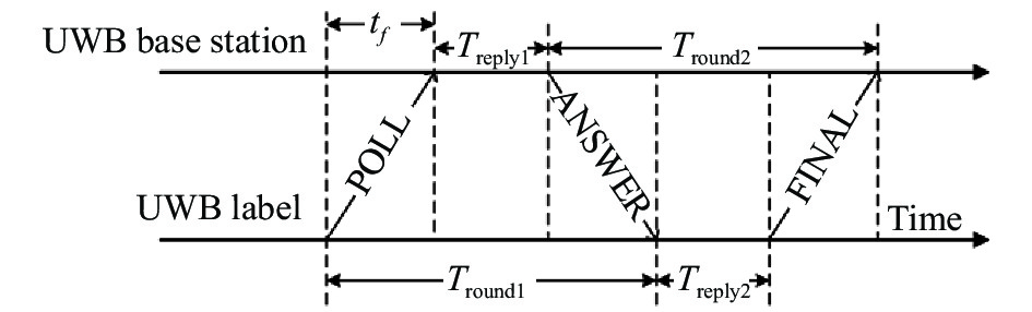
The communication mode of UWB ranging in this paper is shown in Fig. 1.

The UWB label first broadcasts a UWB signal POLL and records the sending time ${T_{a1}}$. After time period ${t_f}$, the signal arrives at the UWB base station. The base station records the time upon receiving the POLL signal ${T_{b1}}$ and continues with signal processing. After time period ${T_{reply1}}$, the base station sends a response signal ANSWER to the label at time ${T_{b2}}\left( {{T_{b2}} = {T_{b1}} + {T_{reply1}}} \right)$. After the label has successfully receives the base station's ANSWER, it then records the reception time ${T_{a2}}$ and sends a FINAL signal after time period ${T_{reply2}}$. After the base station receives the FINAL signal, estimate the transmission time according to the timestamp of each reception time point.

$\left\{ $$\begin{array}{l}{T}_{round}=T_{a2}-T_{a1}\\ T_{reply}=T_{b2}-T_{b1}\\ {\stackrel{⌢}{t}}_f=\left(T_{round}-T_{reply}\right)/2\end{array}$$ \right.$ (1)

Due to variations in attitudes, indoor magnetic fields and environmental layout will all impact the ranging results in different ways when UWB is applied in various environments. To ensure the precision of ranging, it is necessary to calibrate UWB according to the positioning environment.

In the experimental environment, the UWB label is placed with a spacing of 0.1 m, and 30 sets of data are measured in a range of 0.1 m to 3.0 m from the UWB base station. To ensure the precision of the calibration, 1 000 ranging data points are obtained at each distance. The mean values of ranging data collected at each distance are plotted against the actual distances, as shown in Fig. 2.

As shown in Fig. 2, with the increase of the ranging distance, the ranging error shows a decreasing trend, with the maximum ranging error at 0.1 m of 0.47 m.

Take the mean value of ranging data of each distance as the abscissa data and the actual distance as the ordinate data for curve fitting. Tab. 1 shows the root mean square error corresponding to each fitting curve.

As shown in Tab. 1, compared with the quadratic fitting curve and cubic fitting curve, the root mean square error of the quartic fitting curve remains relatively small, and that of the quintic fitting curve is the smallest. Even though the root mean square error of the quantic fitting curve is smaller than that of the quartic fitting curve, the improvement is quite small. Considering the ranging precision and real-time performance, this paper adopts the quartic fitting polynomial as the fitting function of the UWB ranging calibration. The specific fitting function is shown in Equation (2).

$y = 0.029\;87{x^4} - 0.010\;73{x^3} - 0.504\;6{x^2} + 0.910\;8x + 1.544$ (2)

Figure 3 shows the quartic fitting curve.

Figure 4 shows the comparison between actual errors and errors after fitting.

As shown in the figure above, the average ranging error in the 30 ranging data groups before calibration is 0.120 m, while that after calibration fitting is merely 0.012 m. The ranging error of UWB is effectively suppressed by ranging calibration.

According to the ranging data obtained in the calibration process, the overall precision of the ranging is about 0.1 m. However, there are outliers with significant errors in the set of ranging values. Figure 5 (a) and (b) show the data samples of 1 m and 2.5 m ranging in the calibration process, respectively.

In the case of a small number of ranging samples, outliers greatly impact the ranging errors, which subsequently affects the trajectory tracking precision of the positioning target. Therefore, this paper adopts an outlier detection method based on Mahalanobis distance to eliminate the outliers in the UWB ranging process.

The conventional Mahalanobis distance outlier detection method directly applies sample data mean and covariance matrix for calculating the Mahalanobis distance. In the case of a small sample size or a large number of outliers, this method deviates the calculated mean and covariance matrix towards the outliers, resulting in outliers being detected as normal values, futher resulting in incomplete exclusion of outliers. This paper proposes an improvement based on the conventional Mahalanobis distance outlier detection method. In this paper, all mean values and covariance matrixes applied in the detection process are stable values calculated in the Minimum Covariance Determinant (MCD) estimates, so that there is a significant difference between the Mahalanobis distance of the outliers and the normal values in the calculated sample, thereby making it possible to exclude the outliers.

The conventional Mahalanobis distance is calculated with the following equation.

$\left\{ $$\begin{array}{l}d=\sqrt{B^{\mathrm{T}}{S}^{-1}B}\\ B=\left[x_i-T\right]\end{array}$$ \right.$ (3)

Where, d is the Mahalanobis distance, ${x_i}$ is the sample size, T is the mean value of the sample data, and S is the covariance matrix of the sample data. The Mahalanobis distance of the collected sample data is approximately in a chi-square distribution with a degree of freedom of p, and a threshold $\sqrt {x_{p,\alpha }^2} $ is set to a certain confidence coefficient. When the Mahalanobis distance of a calculated ranging value is greater than the set threshold, i.e., $d > \sqrt {x_{p,\alpha }^2} $, it is regarded as an outlier and therefore immediately excluded from the data set ^[9].

The core idea of the modified Mahalanobis distance outlier detection method is to apply FAST MCD algorithm (FAST-MCD) proposed by Rousseeuw^[9], in combination with the conventional Mahalanobis distance calculation process for a stable covariance matrix as well as a stable mean vector, and then calculate the stable Mahalanobis distance according to the conventional Mahalanobis distance equation for eliminating outliers.

First, randomly select a number of $h$ distance data from the distance samples, where $h = M{\rm{ \times }}\alpha $ (0.5< $\alpha $<1), calculate the mean value ${T_1}$ and covariance ${S_1}$ of the $h$ random distance data, and then apply Equation (1) to calculate the Mahalanobis distance $d$ between the $M$ distance samples and ${T_1}$. After that, select $h$ data samples with the minimum Mahalanobis distance from the $M$ distance samples, and calcute the new mean value ${T_2}$ and covariance ${S_2}$ based on the newly selected sample data. ${S_1} = {S_2}$ is only true when ${T_1} = {T_2}$ and $\det \left( {{S_1}} \right) = \det \left( {{S_2}} \right)$. Keep iterating this process until ${T_i} = {T_{i - 1}}$ and ${S_i} = {S_{i - 1}}$. ${T_i}$ and ${S_i}$ obtained at this moment are considered as the stable mean and covariance. Finally, calculate the Mahalanobis distance of each data in the distance sample based on ${T_i}$ and ${S_i}$ with Equation (3), completing the detection of outliers.

The flow chart of the outlier detection method based on the modified Mahalanobis distance is shown in Fig. 6.

Figure 7(a) and (b) show the ranging results at 1 m and 2.5 m upon the exclusion of the outliers by the outlier detection method based on the modified Mahalanobis distance.

As shown in the above two figures, there are no outliers with relatively large deviations in the whole ranging process, and the ranging values demonstrate quite small fluctuations with strong robustness. The above mentioned ranging experiment has demonstrated the effectiveness of the outlier detection method based on the modified Mahalanobis distance adopted in this paper, and that this method is able to ensure real-time ranging while effectively avoiding the occurrence of outliers in the ranging process.

The inertial navigation technology is a fully independent navigation and positioning method. As it has no photoelectric connection with the external environment, it features strong anti-interference capability, high real-time navigation data update rate and excellent stability. However, the errors in the positioning process accumulate over time, which is mainly due to inherent precision of the accelerometer sensor and the gyroscope sensor, thereby making it difficult to position for a prolonged period of time. In current applications, the most effective method to solve this problem is fusion positioning and the use of different sensors to complement each other so as to improve navigational positioning precision^[10].

Compared with common indoor wireless positioning technologies such as WiFi, Bluetooth and ZigBee, UWB signals are advantageous in that they have excellent anti-interference ability, high resolution, centimeter-level ranging accuracy, etc., making UWB signal standing out in the field of wireless positioning^[11]. However, due to the high environmental complexity and large number of obstacles in the case of indoor conditions, the signals may encounter issues such as non-line-of-sight and multi-path during transmission.

In view of the above considerations, this paper designs a UWB and inertial navigation fusion positioning method based on the extended Kalman filter technology, and leverage the strengths and characteristics of both types of sensors, so that they are integrated to complement each other. Therefore, inertial navigation posture is applied to minimize errors caused by the environmental interference in UWB, in addition, the advantage of high precision ranging of UWB is taken to suppress the cumulative error in the inertial navigation solution process.

The fusion positioning method consists of loose coupling and tight coupling depending on the degree of fusion, of which loose coupling is relatively simple. The two systems involved in fusion positioning are independent of each other in the positioning process. Simple fusion is performed on the two sets of positioning results obtained^[12]. On the contrary, tight coupling is a relatively advanced fusion method, where information obtained by the two systems is fused in the process of positioning solution to take full advantages of both, making it an integrated positioning method ^[13-14]. This paper adopts the tight-coupling fusion method, where the UWB ranging data and inertial navigation data are combined to minimize positioning errors.

Generally IMU is fixed to the carrier, so the output data of the sensor is measured in the carrier coordinate system. Therefore, a transformation matrix must be applied to convert the IMU output data into the format in the navigation coordinate system to facilitate calculation. The following section introduces each and every coordinate system adopted in this paper.

(1) Carrier coordinate system

The inertial navigation itself defines an inertial reference coordinate system. However, for the convenience of calculation, when the inertial navigation and the carrier are fixed together, the coordinate system defined by the inertial navigation itself is generally superimposed with the carrier coordinate system. Therefore, when the two coordinate systems are superimposed, the center of mass of the carrier can be taken as the origin of the carrier coordinate system. The X-axis is in the longitudinal direction, that is, the forward direction of the carrier motion. The Z-axis is in the direction perpendicular to the plane of the carrier, and the Y-axis is in a right-handed coordinate system, perpendicular to the XZ plane and pointing to the right. The inertial navigation accelerometer and gyroscope then output the linear acceleration and angular velocity of the carrier moving along the three axes of the carrier coordinate system. The carrier coordinate system in use, also known as the b system, is denoted by $o{x_b}{y_b}{z_b}$. The schematic diagram is shown in Fig.8.

(2) Navigation coordinate system

The navigation coordinate system, also known as the n system, is a global coordinate system for constructing the whole positioning system denoted by coordinates $o{x_n}{y_n}{z_n}$. The navigation coordinate system in this paper is constructed with reference to the UWB base station in indoor positioning environments. The schematic diagram is shown in Fig. 9.

The ground plane in the indoor environment is the XY plane. The Z-axis is a right-handed coordinate system, perpendicular to the XY plane and pointing upwards. The base stations are placed along various coordinate axes, and the origin is where base station 0 is located.

In this paper, EKF is applied to for the tight-coupling fusion positioning of the inertial navigation system and UWB. The functional block diagram of the tight-coupling fusion positioning of the UWB ranging and inertial navigation system is shown in Fig.10.

Pseudorange ${D_S}$ is obtained by applying the position coordinates obtained by UWB base station with known coordinates and SINS calculation. ${D_S}$ is compared with the UWB ranging value ${D_U}$ and is used as the observed value of the system. The error of the system state is estimated based on EKF, and the system state quantity is corrected accordingly.

Given the dynamic characteristics of the positioning target, the system state vectors taken are the 12 dimensions including position, velocity, direction and angular velocity. Before using EKF to estimate the state quantity of the system, estimations of the system state are divided into two parts: estimation of angular velocity and estimation of other system state quantities. Among them, the output of the gyroscope is directly applied as the estimation for the angular velocity, i.e.:

${\overset{\frown} \omega } = {{\textit{z}}_{gyro}}$ (4)

The gyroscope errors consist of scale errors and dynamic errors. Assuming that the gyroscope applied by the system has been well calibrated, all such errors can be ignored, and therefore the output of the gyroscope can be modeled as:

${{\textit{z}}_{gyro}} = \omega + {\eta _{gyro}}$ (5)

In the equation above, ${\eta _{gyro}}$ denotes random noise of the gyroscope.

Similar to the modeling process of the gyroscope, the accelerometer is modeled as:

$a = \ddot X - g + {\eta _{acc}}$ (6)

In the equation above, $a$ denotes the output data directly obtained from the accelerometer, which is the real acceleration of the target, $g$ denotes the gravity acceleration component, and ${\eta _{acc}}$ denotes the random noise of the accelerometer.

Therefore, it only requires to make use of EKF to estimate other system states, namely, estimating a total of state quantities in 9 dimensions, including position, velocity and direction. As the computational complexity of Kalman filter is approximately ${n^3}$ ( $n$ is the dimension of the state vector) ^[15], the computational complexity of the whole Kalman filter process is reduced by more than 50%.

Therefore, in the process of EKF calculation, the state vector $\xi \left( k \right)$ is taken as:

$\xi \left( k \right) = \left( $$\begin{array}{l}X\\ \rho \\ \delta \end{array}$$ \right) = \left( {$$\begin{array}{c}xy\mathit{\text{z}}{\rho }_x{\rho }_y{\rho }_z{D}_0{D}_1{D}_2\end{array}$$} \right)$ (7)

In the equation above, X denotes the position coordinates of the positioning target in the navigation coordinate system, $\rho $ denotes the velocity of the positioning target in the carrier system, and the three-dimensional vector represents the attitude error of the positioning target.

The orientation of the target here is represented by reference attitude and rotation vector $\delta $, among which the magnitude of $\delta $ denotes the rotation angle and the unit vector in the direction of $\delta $ denotes the rotation axis, and the corresponding rotation matrix is denoted by $\exp \left( { [\kern-0.15em[ \delta ]\kern-0.15em] } \right)$.

$ [\kern-0.15em[ \delta ]\kern-0.15em] $ is the skew symmetric matrix of the vector $\delta $:

$\delta = \left( {$$\begin{array}{ccc}{D}_0& D_1& D_2\end{array}$$} \right)$ (8)

$ [\kern-0.15em[ \delta ]\kern-0.15em] = \left[ {$$\begin{array}{ccc}0& D_2& -D_1\\ -D_2& 0& D_0\\ D_1& -D_0& 0\end{array}$$} \right]$ (9)

Expand the first order of $\exp \left( { [\kern-0.15em[ \delta ]\kern-0.15em] } \right)$ as follows:

$\exp \left( { [\kern-0.15em[ \delta ]\kern-0.15em] } \right) = \left( {I + [\kern-0.15em[ \delta ]\kern-0.15em] } \right)$ (10)

Where, I is the identity matrix of size 3 × 3.

The attitude estimation of the positioning target ${\overset{\frown} R} $ can be expressed as follows^[16]:

${\overset{\frown} R} = {{\overset{\frown} R} _{ref}}\left( {I + [\kern-0.15em[ {\overset{\frown} \delta } ]\kern-0.15em] } \right)$ (11)

In the equation above, the reference attitude ${{\overset{\frown} R} _{ref}}$ will be updated according to the rotation vector ${\overset{\frown} \delta } $ after each Kalman filtering estimation, assuming that the reference attitude before the update is denoted by ${{\overset{\frown} R} _{ref,pre}}$, and the reference attitude updated after the Kalman filtering is denoted by ${{\overset{\frown} R} _{ref,post}}$, then

${{\overset{\frown} R} _{ref,post}} = \exp \left( { [\kern-0.15em[ \delta ]\kern-0.15em] } \right){{\overset{\frown} R} _{ref,pre}}$ (12)

${\overset{\frown} \delta } $ is reset to zero after the update of ${{\overset{\frown} R} _{ref}}$^[17].

Assuming that the position change of the internal positioning target relative to the carrier coordinate system during $\Delta t$ (from discrete time k to time (k+1)) is $\Delta X = \left( {\Delta {x^b},\Delta {y^b},\Delta {{\textit{z}}^b}} \right)$, then:

$\left\{ $$\begin{array}{l}\mathrm{\Delta }{x}^b={\rho }_{x,k}\mathrm{\Delta }t+{\displaystyle \frac{1}{2}}{a}_{x,k}\mathrm{\Delta }{t}^2\\ \mathrm{\Delta }{y}^b={\rho }_{y,k}\mathrm{\Delta }t+{\displaystyle \frac{1}{2}}{a}_{y,k}\mathrm{\Delta }{t}^2\\ \mathrm{\Delta }{\mathit{\text{z}}}^b={\rho }_{\mathit{\text{z}},k}\mathrm{\Delta }t+{\displaystyle \frac{1}{2}}{a}_{\mathit{\text{z}},k}\mathrm{\Delta }{t}^2\end{array}$$ \right.$ (13)

R is expressed as the following:

$R = \left[ {$$\begin{array}{ccc}{R}_{00}& R_{01}& R_{02}\\ R_{10}& R_{11}& R_{12}\\ R_{20}& R_{20}& R_{22}\end{array}$$} \right]$ (14)

The position of the target in the navigation coordinate system at time (k+1) is then:

$\left\{ $$\begin{array}{l}{x}_{k+1}=x_k+R_{00}\mathrm{\Delta }{x}^b+R_{01}\mathrm{\Delta }{y}^b+R_{02}\mathrm{\Delta }{\mathit{\text{z}}}^b\\ y_{k+1}=y_k+R_{10}\mathrm{\Delta }{x}^b+R_{11}\mathrm{\Delta }{y}^b+R_{12}\mathrm{\Delta }{\mathit{\text{z}}}^b\\ {\mathit{\text{z}}}_{k+1}={\mathit{\text{z}}}_k+R_{20}\mathrm{\Delta }{x}^b+R_{21}\mathrm{\Delta }{y}^b+R_{22}\mathrm{\Delta }{\mathit{\text{z}}}^b\end{array}$$ \right.$ (15)

The velocity of the positioning target in the carrier coordinate system at time (k+1) can be obtained from the following equation.

$\left\{ $$\begin{array}{l}{\rho }_{x,k+1}={\rho }_{x,k}+a_{x,k}\mathrm{\Delta }t\\ {\rho }_{y,k+1}={\rho }_{y,k}+a_{y,k}\mathrm{\Delta }t\\ {\rho }_{\mathit{\text{z}},k+1}={\rho }_{\mathit{\text{z}},k}+a_{\mathit{\text{z}},k}\mathrm{\Delta }t\end{array}$$ \right.$ (16)

The update of $\delta $ can be obtained from the following equation.

${\delta _{k + 1}} = \exp \left( { [\kern-0.15em[ d ]\kern-0.15em] } \right){\delta _k}\exp {\left( { [\kern-0.15em[ d ]\kern-0.15em] } \right)^{\rm T}}$ (17)

In the above equation, d denotes the attitude error represented by the Rodriguez parameter, as follows:

$d = \left( {{d_0},{d_1},{d_2}} \right) = \left( {\frac{{{\omega _x}dt}}{2},\frac{{{\omega _y}dt}}{2},\frac{{{\omega _z}dt}}{2}} \right)$ (18)

${\omega _x}$, ${\omega _y}$, ${\omega _z}$ are the angular velocity of the gyroscope relative to the three axes of the carrier coordinate system in discrete time interval, and are regarded as constants within the sampling time.

The state model of the system is expressed as follows:

${{\overset{\frown} \xi } _{k + 1}} = f\left( {{{{\overset{\frown} \xi } }_k}} \right)$ (19)

f in the equation above represents the linearized function model after first order Taylor expansion of the system.

In UWB and inertial navigation fusion positioning, since the UWB ranging has no cumulative errors and the ranging error is merely around 0.1 m, it falls into the wireless ranging technology with relatively high precision. Therefore, UWB ranging values are used as the observed values of extended Kalman filtering.

One assumption is that the coordinates at known position ${p_i}$ of the UWB base station are $\left( {$$\begin{array}{ccc}{p}_{i,x}& p_{i,y}& p_{i,\mathit{\text{z}}}\end{array}$$} \right)$, and the ranging value obtained by using UWB label at time k is ${d_{i,k}}$. The other assumption is that the actual position coordinate of the positioning target is ${X_k} = \left( {{{$$\begin{array}{ccc}{x}_k& y_k& {\mathit{\text{z}}}_k\end{array}$$}}} \right)$. Therefore, the observation equation can be modeled as:

${d_{i,k}} = \left\| {X - {p_i}} \right\| + {\nu _d}$ (20)

Where, ${\nu _d}$ denotes the process noise of the UWB measurements, and $ \Vert \cdot \Vert $denotes the Euclidean norm, also known as Euclidean distance, therefore:

$ \left\| {X - {p_i}} \right\| = \sqrt {{{\left( {{x_k} - {p_{i,x}}} \right)}^2} + {{\left( {{y_k} - {p_{i,y}}} \right)}^2} + {{\left( {{z_k} - {p_{i,z}}} \right)}^2}} $ (21)

And the observation matrix is:

${H_i} = \dfrac{{\partial {d_{i,k}}}}{{\partial \xi }} = \left( {$$\begin{array}{ccc}{\displaystyle \frac{\partial d_{i,k}}{\partial X}}& {\displaystyle \frac{\partial d_{i,k}}{\partial \rho }}& {\displaystyle \frac{\partial d_{i,k}}{\partial \delta }}\end{array}$$} \right)$ (22)

Where,

$\left\{ $$\begin{array}{l}{\displaystyle \frac{\partial d_{i,k}}{\partial X}}={\displaystyle \frac{X-p_i}{\Vert X-p_i\Vert }}\\ {\displaystyle \frac{\partial d_{i,k}}{\partial \rho }}={\displaystyle \frac{\partial d_{i,k}}{\partial \delta }}=0\end{array}$$ \right.$ (23)

In the above equation, $\dfrac{{X - {p_i}}}{{\left\| {X - {p_i}} \right\|}}$ can be expressed as an identity vector ${e_i}$. And the observation matrix is found as a sparse matrix.

Assuming that the position coordinate obtained by the solution of the positioning target is ${\tilde X_k} = \left( {{{\tilde x}_k}}\;\;{{{\tilde y}_k}}\;\;{\tilde {\textit{z}}}_k \right)$, therefore, the prediction equation of the observation is:

${Z_k} = \sqrt {{{\left( {{{\tilde x}_k} - {p_{i,x}}} \right)}^2} + {{\left( {{{\tilde y}_k} - {p_{i,y}}} \right)}^2} + {{\left( {{{\tilde {\textit{z}}}_k} - {p_{i,{\textit{z}}}}} \right)}^2}} $ (24)

Based on the state equation and observation equation, the target state information can be obtained by the time update and state update of the EKF.

The time update equation is:

$\left\{ $$\begin{array}{l}{\stackrel{⌢}{\xi }}_{k+1|k}=f\left({\stackrel{⌢}{\xi }}_{k|k}\right)\\ P_{k+1|k}=\Phi P_{k|k}{\Phi }^{\mathrm{T}}+Q\end{array}$$ \right.$ (25)

State update equation is:

$\left\{ $$\begin{array}{l}{K}_{k+1}=P_{k+1|k}{H}^{\mathrm{T}}{\left(H{P}_{k+1|k}{H}^{\mathrm{T}}+R\right)}^{-1}\\ {\stackrel{⌢}{\xi }}_{k+1}={\stackrel{⌢}{\xi }}_{k+1|k}+K_{k+1}\left(Z_{k+1}-H{\stackrel{⌢}{\xi }}_{k+1|k}\right)\\ P_{k+1}=\left(I-K_{k+1}H\right)P_{k+1|k}\end{array}$$ \right.$ (26)

The experimental test environment in this paper is a laboratory with a size of 5.0 m×8.0 m. Positioning cameras with the Optitrack high-precision positioning motion capturing system are set around a 4.0 m×4.2 m rectangle in the room. The experiment site in this paper is located in a 2.4 m×2.4 m rectangle within the motion capturing system. The motion capturing system is a high-precision indoor positioning system adopting infrared cameras to cover indoor positioning space. Reflective markers are placed on the objects to be positioned. The three-dimensional position information of these objects is calculated by capturing the reflection images of the reflective markers on the positioning cameras. In addition, the precision of the Optitrack positioning cameras is as high as 0.1 mm. In all experiments in this paper, trajectories calculated based on the motion capturing system are taken as actual target trajectories, the positioning precisions of which are compared with the proposed positioning method in this paper.

In the experimental scene of this paper, six UWB base stations are set up and labelled with ID 0 to 5, respectively. The main control chip applied by the UWB base station is STM32F103RC.

The layout of the UWB base stations in the experimental environment and the navigation coordinate system used in this paper are shown in Fig. 11.

In measuring the coordinates of the base stations, the reflective markers identifiable by the motion capturing system are first placed on the base stations, and then the positioning coordinates captured by the motion capturing system are taken as specific position coordinates of each base station, as shown in Tab. 2.

To verify the precision of the UWB and inertial navigation fusion positioning method proposed in this paper, field experiments are carried out, the estimated trajectory errors, the positioning accuracy and trajectory error of the two positioning methods are calculated.

As shown in Fig.12, in this experiment, the positioning label is fixed to a positioning trolley. The trolley is controlled by the motion capturing system based on the feedback of the input trajectory coordinates. In the experiment, the trolley moves at a speed of 0.05 m/s, and the motion precision of the trolley is up to centimeter level at this speed. The positioning label affixed to the trolley is supplied by a power bank via a USB port. A reflective marker point identifiable by the motion capturing system is laid on the center of the positioning label.

The controlled trolley moves in a rectangular track of 1.2 m×1.2 m at the experiment site. The schematic diagram of the simulated trolley trajectory is shown in Fig.13. The trolley began its trajectory at point A and moved 1.2 m to point B, after which it further moves 1.2 m to point C and 1.2 m to point D until it eventually returns to point A. In the experiment results, the trajectory of the reflective marker in the center of the positioning label obtained by the motion capturing system is taken as the actual motion trajectory of the positioning label.

First, the ranging data obtained in the movement of the trolley is input into MATLAB and the UWB positioning trajectory was generated. The results are shown in Fig.14(a) and (b).

In Fig.14(a) and (b), the line formed by red dots represents the actual motion trajectory, and the solid blue line represents the position trajectory only with UWB for positioning. An artificial disturbance is added during the trolley motion by human movement, creating obstruction between the UWB base stations and the label. According to the experiment data, better motion trajectories of the positioning target are obtained by applying UWB without obstruction. In segments A B, B C and D A before introducing obstruction, the maximum positioning error and the mean absolute error are 0.461 m and 0.378 m, respectively, which has achieved positioning at centimeter level. However, in segment C D with human interference introduced, the maximum positioning error is 1.153 m, and the mean absolute error is 0.412 m. Throughout the rectangular trajectory experiment, the maximum absolute error is 1.153 m, the mean absolute error is 0.386 m, and the root mean square error is 0.397 m. Based on the above data, that obstructions of the UWB signal have no great impact on the precision of the final positioning. In this case, the positioning results by applying UWB and inertial navigation fusion are given below in Fig.15(a) and (b).

In Fig.15(a) and (b), the line formed by red dots represents the actual motion trajectory, the solid blue line is the motion trajectory obtained with UWB alone for the positioning experiment, and the black double dashed line is the motion trajectory with the UWB and inertial navigation fusion method. It can be seen from the figure that, compared to the positioning only with UWB, the positioning using the fusion of UWB and inertial navigation can achieve a higher positioning accuracy without changing the real-time performance.

Figure 16 and Fig.17 show error comparison of the two positioning methods.

As can be seen from Fig.16, even though a surge of errors in positioning with UWB and inertial navigation fusion is observed in case of interference, the errors are significantly reduced compared with the positioning results only with UWB. Robustness of positioning is significantly improved.In the positioning with UWB and inertial navigation fusion, in segments A B, B C and D A before introducing the obstruction, the maximum positioning error is 0.305 m, and the mean absolute error is 0.232 m, which has enabled positioning at centimeter level. However, in segment C D with human interference introduced, the maximum positioning error is 0.692 m, and the mean absolute error is 0.285 m. Throughout the rectangular trajectory, the mean absolute error is 0.246 m and the root mean square error is 0.255 m, demonstrating that such positioning method has reached a high positioning precision. Compared with the positioning results with UWB alone, the mean precision is improved by 36.3% and the root mean square error is reduced by 35.8%.

According to Fig.17, when UWB alone is used for positioning, the error is within 1.0 m, and around 90% of the points have an error of 0.4 m, while the error of the UWB and inertial navigation fusion positioning is within 0.6 m, and over 90% of the points have an error of less than 0.25 m.

To achieve the goal of obtaining high-precision positioning information of positioning labels in complex indoor environments, this paper studies the fusion positioning method by applying UWB and inertial navigation. First, calibrate the UWB ranging in the experimental environment. Then, detect and eliminate outliers with an outlier detection algorithm based on modified Mahalanobis distance. And finally, based on the extended Kalman filter algorithm, design and program an indoor fusion positioning method with UWB technology and inertial navigation system. Perform experimental validation and analyze the experiment in the experimental environment. The final experimental results show that the method proposed in this paper has higher accuracy and better robustness compared with those of the traditional single-sensor positioning method.

Nevertheless, this study only introduces the single external interference, which would generally develop into a variety of interferences in actual application scenarios. Therefore, the current algorithms are subject to optimization in future works, with detailed work as follows.

(1) Extend the positioning environment, consider a method that can dynamically select UWB base stations in the environment, and further improve the accuracy of UWB ranging.

(2) Consider the introduction of more complex interference models, and focus on the research on more fusion related methods, such as applications of particle filtering and factor graph in fusion positioning algorithms.

(3) Introduce more sensors to the positioning system, and design a fusion positioning system with both UWB and multi-sensor.

References

[1] M Uradzinski, H Guo, X Liu, et al. Advanced indoor positioning using Zigbee wireless technology. Wireless Personal Communications, 97, 6509-6518(2017).
[2] A Oulose, O S Eyobu, D S Han. An indoor position estimation algorithm using smartphone IMU sensor data. IEEE Access, 7, 11165-11177(2019).
[3] Y L Wang, J N Lv, J H Li, et al. High precision indoor positioning system based on UWB. Yangtze River Information Communication l, 34, 111-114, 117(2021).
[4] Chen D L, Yang Z. Study on high precision indo positioning technology based on UWBMEMS[D]. Xuzhou: China University of Mining Technology, 2015.(in Chinese)
[5] B W Sun, Q G Fan, Y H Wu, et al. Foot-mounted pedestrian navigation technology based on tightly coupled PDR/UWB. Transducer and Microsystem Technologies, 36, 43-48(2017).
[6] Zampella F, Angelis A D, Skog I, et al. A constraint approach f UWB PDR fusion[C]Proceedings of the 2012 International Conference on Indo Positioning Indo Navigation (IPIN), IEEE, 2012: 26.
[7] L L Chen, Y Yang, E Yuan, Y X Zhao, et al. Integrated indoor positioning algorithm based on UWB/PDR. Information Technology and Network Security, 38, 53-57(2019).
[8] Alhadrami S, Salman A, Khalifa H A. Ultra wideb positioning: an analytical study of emerging technologies[C]Proceeding of International Conference Sens Technologies Applications (SENSCOMM). IEEE, 2014: 19.
[9] P Q Yin, D M Lu, Y Yuan, et al. An improved non-local image de-noising algorithm based on Mahalanobis distance. Journal of Computer-Aided Design & Computer Graphics, 28, 404-410(2016).
[10] Hailiang Xiong, Ruochen Bian, Yujun Li, et al. Fault-Tolerant GNSS/SINS/DVL/CNS integrated navigation and positioning mechanism based on adaptive in-formation sharing factors. IEEE Systems Journal, 14, 3744-3754(2020).
[11] Kai Wen, Kegen Yu, Yingbing Li. A new quaternion Kalman filter based foot-mounted IMU and UWB tightly-coupled method for indoor pedestrian navigation. IEEE Transactions on Vehicular Technology, 69, 4340-4352(2020).
[12] Q L Tian, K I K Wang, Z Salcic. A resetting approach for INS and UWB sensor fusion using Particle Filter for pedestrian tracking. IEEE Transactions on Instrumentation and Measurement, 69, 5914-5921(2020).
[13] her C, Zwirello L, Zwick T, et al. Integrity moniting f UWBINS tightly coupled pedestrian indo scenarios [C]Indo Positioning Indo Navigation (IPIN), 2011 International Conference on. IEEE, 2011, PP(16): 6071948.
[14] Hailiang Xiong, Zhenzhen Mai, Juan Tang, et al. Robust GPS/INS/DVL navigation and positioning method using adaptive federated strong tracking filter based on weighted least square principle. IEEE Access, 7, 26168-26178(2019).
[15] BarShalom Y, Li X R, Kirubarajan T. Estimation with Applications to Tracking Navigation: They Algithms Software[M]. Canada: John Wiley & Sons, 2001: 303306.
[16] Zipfel P H. Modeling Simulation of Aerospace Vehicle Dynamics[M]. 2nd ed. USA: American Institute of Aeronautics Astronautics, 2007: 98101.
[17] F L Markley. Attitude error representations for Kalman filtering. Journal of Guidance, Control, and Dynamics, 26, 311-317(2003).
Set citation alerts for the article
Please enter your email address
© Copyright 2018-2021 | Chinese Laser Press. All Rights Reserved 沪ICP备15018463号-20