
Baijun Li, Ran Huang, Xunwei Xu, Adam Miranowicz, Hui Jing, "Nonreciprocal unconventional photon blockade in a spinning optomechanical system," Photonics Res. 7, 630 (2019)
- Photonics Research
- Vol. 7, Issue 6, 630 (2019)
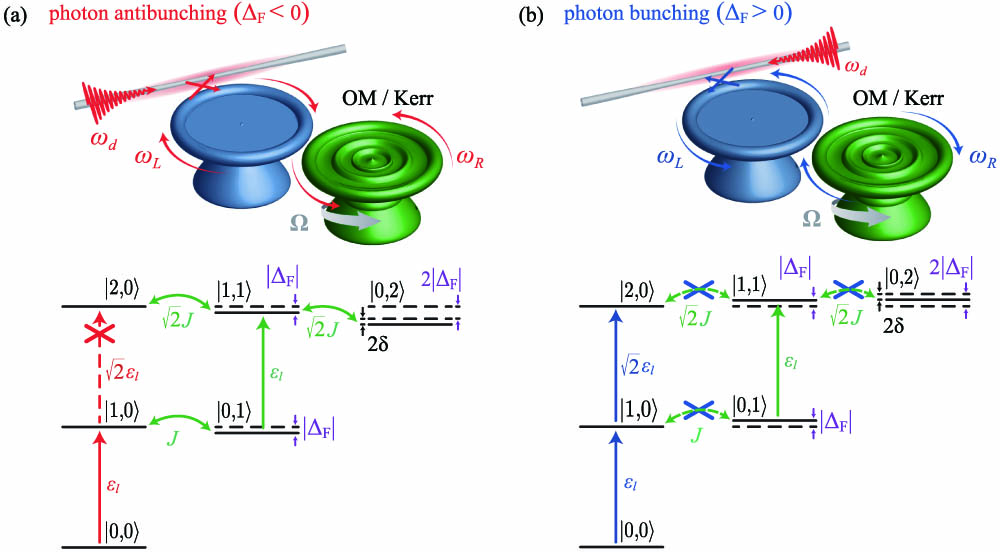
Fig. 1. Nonreciprocal UPB in a coupled-resonator system. Spinning the OM (Kerr-type) resonator results in different Fizeau drag Δ F | 1 , 0 ⟩ | 2 , 0 ⟩ δ = g 2 / ω m
![Correlation function gL(2)(0) versus optical detuning Δ/κ (in units of cavity loss rate κL=κR=κ) with (a) Ω=0 and (b) Ω=12 kHz, which is found numerically (solid curves) and analytically (dotted curve). The PB can be generated (red curves) or suppressed (blue curves) for different driving directions, which can be seen more clearly in panel (c). The other parameters are g/κ=0.63, ωm/κ=10 [91], J/κ=3, T=0.1 mK (case 1), and g/κ=0.1 [28], ωm/κ=30 [92], J/κ=20, T=1 mK (case 2).](/richHtml/prj/2019/7/6/06000630/img_002.jpg)
Fig. 2. Correlation function g L ( 2 ) ( 0 ) Δ / κ κ L = κ R = κ Ω = 0 Ω = 12 kHz g / κ = 0.63 ω m / κ = 10 J / κ = 3 T = 0.1 mK g / κ = 0.1 ω m / κ = 30 J / κ = 20 T = 1 mK
Fig. 3. Correlation function g L ( 2 ) ( 0 ) Δ / κ κ L = κ R = κ Ω 12 ), whereas the solid curves are our numerical solutions. The other parameters are the same as those in Fig. 2 (case 1).
Fig. 4. Correlation function g L ( 2 ) ( 0 ) log 10 g L ( 2 ) ( 0 ) g / κ κ = κ L = κ R Δ / κ J / κ g / κ Δ / κ = − 0.05 Ω = 12 kHz g L ( 2 ) ( 0 ) = 1 3 .
Fig. 5. Correlation function g L ( 2 ) ( 0 ) Δ / κ κ L = κ R = κ n Ω Δ F 4 .
Fig. 6. (a) Correlation function g L ( 2 ) ( 0 ) T Δ F Δ F > 0 Δ F = 0 Δ F < 0 Δ opt g opt 2 . Also shown is the correlation function g L ( 2 ) ( 0 ) T


Set citation alerts for the article
Please enter your email address

© Copyright 2018-2021 | Chinese Laser Press. All Rights Reserved 沪ICP备15018463号-20