
Simon Roeder, Yannik Zobus, Christian Brabetz, Vincent Bagnoud, "How the laser beam size conditions the temporal contrast in pulse stretchers of chirped-pulse amplification lasers," High Power Laser Sci. Eng. 10, 06000e34 (2022)
- High Power Laser Science and Engineering
- Vol. 10, Issue 6, 06000e34 (2022)
Abstract
1 Introduction
The temporal profile of short laser pulses generated by high-intensity lasers exhibits complex features commonly referred to as ‘temporal contrast’. The issue of temporal-contrast degradation has been studied ever since the invention of the chirped-pulse amplification (CPA) technique[1] because of its deleterious effect on high-intensity-laser-driven experiments. Temporal-contrast mitigation methods palliating the problem[2] were first proposed, but these systematically increase the complexity of the laser architecture by adding pulse-cleaning stages, either in the front-end of the laser[3–5] or after the pulse compressor at the back-end of the laser[6–9]. Alternatively, temporal-pedestal-free amplifiers[10] can be designed to replace the first stage of amplification in CPA lasers to keep the temporal contrast in check without adding complexity to the system[11]. As a consequence, the temporal contrast becomes less and less limited by pedestals on the ns-scale and prepulses. Instead the temporal contrast is now mainly limited by a slow rising edge on the ps-scale, which can be observed systematically at laser facilities all around the world[12–16]. While the effect of the slow rising edge is not as stringent as that of the nanosecond pedestal, it is still a major problem for laser–plasma interaction experiments, as the interaction of such a profile with targets remains difficult to predict and it is thus a large source of uncertainty.
During the past two decades, it has been established that this slow rising edge is caused by scattering effects, which are introduced whenever a spectrally dispersed laser pulse is reflected from a surface, such as in the stretcher and the compressor of CPA laser systems. A first indication that surface defects in the pulse stretcher map onto the residual spectral phase and influence the pulse profile was given more than 20 years ago[17]. It took over a decade after the first description of the pulse distortion before a theoretical analysis was provided[18] that generalized this effect to all spatial frequencies of stretcher optics. This, for the first time, utilized the quantification of the surface imperfections that the Fourier decomposition of the surface height distribution, called the power spectral density (PSD), of the relevant surface provides. Even though it is not explicitly stated in the paper, this implies that each such reflection contributes to the rising edge and that the magnitude of it depends on the PSD of the surface. This description still neglected the spatial extension of the beam and assumed the beam to be a 1D line during the propagation throughout the stretcher. Experiments verified this and showed that either the gratings[19] or optics[12] could dominate the temporal-contrast degradation, in a specific setup. In both cases, optical elements of lower scattering and better quality proved to have a beneficial effect on the temporal contrast, increasing it by one to three orders of magnitude.
The incorporation of the beam size into the analytical description was provided by Bromage et al.[20], who focused on spatio-temporal coupling effects due to surface scattering. This model, which neglected diffraction, is adapted to describe large beam sizes like in a pulse compressor. Based on this approach, the authors even proposed an experimental stretcher setup that would prove this theory[21]. Even though we are not aware that they ever followed up on the experimental verification, the theoretical work provided the means to repeat the previously made statement that two optical elements with identical PSD will produce the same rising edge, and expand on this by recognizing that for identical PSDs of the surface, the reflection with the smaller beam size will introduce the larger rising edge.
In a recent work by our group[22], we corroborated the concomitant relation between beam size and stretcher optics defects in phase and amplitude on the temporal contrast, using a 2D self-made ray tracing model that includes diffraction effects. One result indicated that the folding mirror commonly found in the Fourier plane of the stretcher might dominate the rising edge due to the small beam size at this location. A clear implication of this is that the temporal contrast can be improved by increasing the surface quality of this optical element[12] or even completely removing this optical element from the stretcher design, as recently demonstrated by Lu et al.[23,24].
In this work, we propose and validate experimentally a new analytical description of the temporal-contrast degradation based on the beam size and PSD of optical surfaces in a pulse stretcher. Furthermore, we propose to use the beam size as a new method of optical temporal-contrast control that, in comparison with Hooker et al.[19] and Ranc et al.[12], does not only influence the offset of the rising edge, but can also be used to manipulate the steepness of the rising edge.
In the first part, we discuss the analytical derivation of the relationship among beam size, PSD and rising edge. Our model differs from previous approaches found in the literature[18,20] because we consider that beam diffraction and propagation effects throughout the laser amplifier introduce a spatial averaging effect that must be accounted for. Afterwards we discuss the experimental stretcher setup that we used for this proof-of-principle and compare the results with the predictions that can be made using the analytical description. In the last part, we discuss the implications of this for future stretcher designs.
2 Theory
As stated above, the effect that causes the rising edge in the pulse profile is the coherent scattering introduced by a disturbed surface acting on a spectrally dispersed laser beam. The spectral dispersion on a surface can be approximated by a linear dependency between the position on the surface and the corresponding angular frequency
In order to find an analytical description of the temporal profile, we will start with a general electrical field of a short laser pulse propagating in a stretcher that can be formulated in the spectral domain as follows:
Assuming that the disturbance
This can be interpreted as the (inverse) Fourier transform from the spatial domain into the spatial frequency domain at the spatial frequency
If we now take the absolute square of this we get the temporal profile of the laser pulse:
Since the imaginary part is multiplied with the Fourier transform of the spectral field
If we now again assume that the variation of
If we now in a last step recognize how the Fourier transform of the height profile
This formula enables us to predict the rising edge of a given experimental setup. It allows the calculation of the rising edge caused by optics in the near-field and in the far-field for various beam sizes and shapes. While this work is concerned with the impact of the in-stretcher beam size on the temporal contrast, it should be noted that Equation (13) depends on the absolute square of the Fourier transform of the spatial profile at the considered optical element. If we consider a mirror in the near-field, the final formula depends on the spatial intensity distribution in the far-field and vice versa. Thus, the wavefront in the near-field directly influences the temporal contrast and aberrations of all kind can cause temporal-contrast degradation. Therefore, it is crucial to control the wavefront in order to investigate the beam size dependence. We will later on use this insight to calculate an uncertainty for the temporal profile. It should be further noted that the PSD, which is originally a function of the spatial frequency of the surface, is expressed here as a function over time. How this mapping can be done is covered in the appendix.
3 Experimental validation
In order to verify our findings, we built a test setup that included a temporally clean short pulse source, a variable stretcher in zero-stretch configuration and a scanning cross-correlator (Sequoia, Amplitude). The short pulses are produced by a commercial oscillator at a center wavelength of 1040 nm (Mira, Coherent), which are then further amplified by a homemade ultrafast optical parametric amplifier (uOPA) to several tens of microjoules and a full width at half maximum (FWHM) bandwidth around 6.2 nm[11]. We were able to resolve the temporal profile of these pulses in the third-order cross-correlator over a dynamic range of nine orders of magnitude, which is sufficient for this analysis.
For the stretcher setup, we decided to use spherical mirrors for the telescope and a flat folding mirror that is positioned in the Fourier plane, as shown in Figure 1. We positioned the gratings at half the radius of curvature too, in order to achieve a zero-stretch configuration. In this way, we were able to measure the temporal profile directly after the stretcher without the need for a compressor. This allows us to isolate the influence of the telescope and the folding mirror.
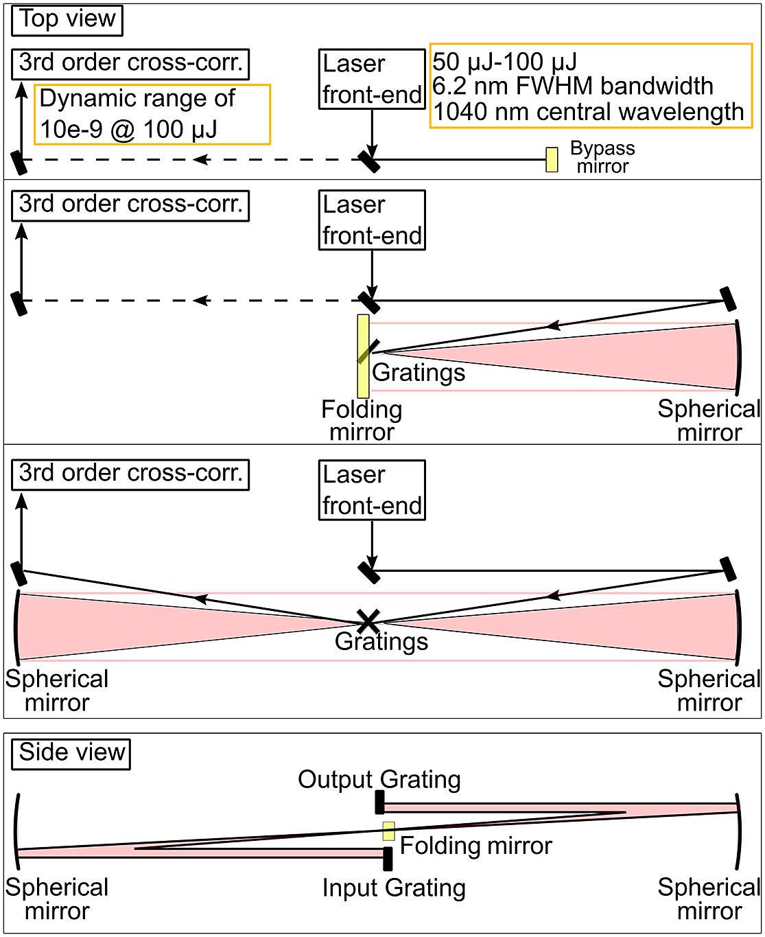
Figure 1.Schematic of the experimental stretcher setup with three configurations. First from the top, the laser pulse bypasses the stretcher using the bypass mirror; second from the top, the beam enters the stretcher, is incident on an optical grating (G) (
 ) and a spherical mirror (
 ), before being reflected from a folding mirror; third from the top, the pulse enters the stretcher and transverses through an unfolded design with two gratings and two spherical mirrors. In all three configurations the beam path ends in the third-order cross-correlator (Sequoia, Amplitude) with which the temporal profile is measured. The very bottom depicts a side view of the general setup.
The downside of this setup is that we cannot investigate the impact of the stretcher gratings since the laser beam is not spectrally dispersed there, but we expect that the rising edge caused by gratings can be described analogously to mirrors. Thus, when investigating the spherical mirror and the folding mirror is sufficient in order to validate the analytical solution provided in this work, this solution allows us to predict the temporal profile for each optical element, even for the gratings. The described configuration would require us to stack two gratings on top of each other, which was cumbersome; thus we introduced a small mirror in the intermediate field between the spherical mirror and the grating. Since the spectral dispersion on this mirror is small, we neglected its impact in the following considerations.
The stretcher, which is depicted in Figure 1, can be either completely bypassed using a mirror on a magnetic mount or in two different configurations. The first of these two configurations is folded with a flat mirror located in the Fourier plane and the second is unfolded, ensuring that the beam size remains equal on all of its optics. All other parameters of the stretcher were kept constant for both configurations, especially the angle of incidence into the stretcher and the grating constant (and thus the spatial-dispersion coefficient
During this experimental campaign, the temporal contrast was measured in all configurations for two different beam sizes. The results of those measurements are summarized in Figure 2, where the background level of each measurement is given by the dynamic range of the cross-correlator. The top figure (Figure 2(a)) depicts the measurements done in the folded design and the bottom figure (Figure 2(b)) depicts the same measurements done in the unfolded configuration. Both configurations were used with a smaller beam size of (1.1 ± 0.05) mm, shown in blue, and with a larger beam size of (5.8 ± 0.5) mm, shown in red. In order to emphasize the change of the slope of the rising edge that is caused by the change in beam size, we included fits to the rising edge for the folded design. Those fits are expressed as black lines, with the steeper one corresponding to the smaller beam size (and thus larger focal spot). It is furthermore noted that the background level varies with the setup. This is due to the limited efficiency of the gratings, which decreases the energy in the pulse and thus the intensity in the cross-correlator. For the larger beam size this is compensated for by a smaller focal spot in the cross-correlator, which leads to a higher intensity. The solution to the analytical approximation is also indicated in the figures, taking into account measurement uncertainties, indicated as shaded areas. In order to calculate these solutions and later on their uncertainties, we had to measure several parameters. Firstly, the undisturbed temporal profile
![]()
Figure 2.Measured temporal profile of a laser pulse that was amplified in a uOPA stage (bypass), after transversing through a folded stretcher (a) or an unfolded stretcher (b). The measurements were executed for a smaller beam size, indicated as blue in the plot (FWHM = 1.1 mm) and a larger beam size, indicated as red in the plot (FWHM = 5.8 mm). Shaded areas indicate uncertainties of the alignment procedure. The black lines indicate the slope of the rising edge, with the steeper line corresponding to the smaller beam.
However, knowing the beam size in the near-field is not enough to assess the beam size in the far-field, where scattering from the folding mirror dominates. Thus, analytical Gaussian beam propagation and geometrical considerations of the impact of the diffraction from the grating onto the beam size and wavefront were used in order to estimate the actual beam sizes at the respective optical elements more accurately. For this we assumed the wavefront to be flat at the position of the CCD camera (a fact that we will reconsider shortly, when we calculate the uncertainty of the calculated rising edge). The incorporation of the beam propagation over a distance of 2 m has a significant impact on the small beam size, but is almost negligible for the large beam size. Lastly, we estimated the PSD of the relevant optics, being the spherical mirror used for the telescope and the planar folding mirror. High spatial resolution data on the surface profile were gathered at the metrology laboratory of CEA-CESTA, France, using a confocal microscope with a magnification between 0.5× and 1×. The results of our PSD analysis are depicted in Figure 3.
![]()
Figure 3.PSD of the spherical mirror and the flat folding mirror used in the stretcher setup, as commonly expressed in variance over frequency interval. Since the variance of the height distribution is approximately of the order of nm and the relevant spatial frequency interval of the order of mm−1, we chose nm2 mm.
Now, for the calculation of the uncertainty of the rising edge we considered that the wavefront might not necessarily be flat at the position of the CCD camera. We substituted the CCD camera with a Shack–Hartmann sensor (SHS). Besides the estimation of the wavefront, this was necessary because we had to align a magnifying telescope for the large beam and compensate diffraction for the small beam. The accuracy of the SHS, which consists of a micro-lens array and a CCD chip, is, without absolute calibration, limited by the specifications of the micro-lens pitch and the size of the CCD chip (or more accurately, the mean distance between the pixels). Uncertainties in these two parameters directly translate to uncertainties in the defocus. We can estimate the uncertainty of the wavefront measured with the SHS to be a defocus of roughly
4 Discussion and conclusion
In this work, we showed how the beam size in the pulse stretcher can condition the rising edge of a laser pulse amplified by CPA. Our simple analytical model describes the interplay between beam size, PSD and temporal profile. This model confirms that the surface PSD of the optical elements is responsible for the rising edge, but that its shape and slope are due to the beam size. In particular, the slope in the stretcher is steeper when the beam size is larger. Furthermore, we conducted an experimental campaign, during which we were able to push the point in time where the rising edge breaches the noise level (for the available energy in this proof-of-principle, it is around 10−9) from 55 to 5 ps, while using off-the-shelf optical components. The value of 55 ps was the best effort contrast for the folded design, which we found at the smallest tested beam size and thus largest focus. For the unfolded design, we observed a switch in the dependency on the beam size, as the roughness of the optical elements in the near-field prevails, yielding a better contrast for the larger beam. In this setup, nine orders of magnitude contrast at 5 ps were achieved, which is a considerable improvement compared with the 55 ps that was possible in the folded setup.
When we compare this with the analytical solutions, we find a good agreement within the measurement uncertainty in the behavior of both experiment and theory, as we can see that the folding mirror and the spherical mirror show an opposing dependency with the size of the beam, which is incident in the stretcher. Currently this model is only valid for beams with an aspect ratio of around one, but it could be adapted to be applicable to elliptical beams by incorporating a second spatial integral into the considerations. A further limit of our analytical model that we find is the cases where, due to a large beam size, the rising edge is fully suppressed to times that are not considerably larger than the pulse length, since the approximation that allowed us to find Equation (10) is not valid in this region. The study of this region furthermore requires a measurement of the PSD over a larger sample size.
A consequence of this work is the necessity to develop new stretcher designs that do not incorporate optical elements in their Fourier plane, and at the same time it gives an analytical formulation that can be used to optimize PSD and beam size to reach a targeted contrast level. Such design rules can be derived from the interplay between the rising edge and the aspect ratio on the surface, which is given by the in-stretcher beam size and the spatial-dispersion coefficient
References
[1] D. Strickland, G. Mourou. Opt. Commun., 55, 447(1985).
[2] J. Itatani, J. Faure, M. Nantel, G. Mourou, S. Watanabe. Opt. Commun., 148, 1(1998).
[3] A. Jullien, O. Albert, F. Burgy, G. Hamoniaux, J.-P. Rousseau, J.-P. Chambaret, F. Augé-Rochereau, G. Chériaux, J. Etchepare, N. Minkovski, S. M. Saltiel. Opt. Lett., 30, 920(2005).
[4] R. C. Shah, R. P. Johnson, T. Shimada, K. A. Flippo, J. C. Fernandez, B. M. Hegelich. Opt. Lett., 34, 2273(2009).
[5] L. Yu, Y. Xu, Y. Liu, Y. Li, S. Li, Z. Liu, W. Li, F. Wu, X. Yang, Y. Yang, C. Wang, X. Lu, R. Li, Z. Xu. Opt. Express, 26, 21626(2018).
[6] H. C. Kapteyn, M. M. Murnane, A. Szoke, R. W. Falcone. Opt. Lett., 16, 490(1991).
[7] C. Ziener, P. Foster, E. Divall, C. Hooker, M. Hutchinson, A. Langley, D. Neely. J. Appl. Phys., 93, 768(2003).
[8] D. Neely, C. Danson, R. Allott, F. Amiranoff, J. Collier, A. Dangor, C. Edwards, P. Flintoff, P. Hatton, M. Harman, M.-H.-R. Hutchinson, Z. Najmudin, D. A. Pepler, I. N. Ross, M. Salvati, T. Winstone. Laser Particle Beams, 17, 281(1999).
[9] D. Hillier, C. Danson, S. Duffield, D. Egan, S. Elsmere, M. Girling, E. Harvey, N. Hopps, M. Norman, S. Parker, P. Treadwell, D. Winter, T. Bett. Appl. Opt., 52, 4258(2013).
[10] C. Dorrer, I. Begishev, A. Okishev, J. Zuegel. Opt. Lett., 32, 2143(2007).
[11] Y. Zobus, C. Brabetz, J. P. Zou, V. BagnoudConference on Lasers and Electro-Optics. , , , and , in (CLEO) (Optica, 2011), paper STh2B.3..
[12] L. Ranc, C. Le Blanc, N. Lebas, L. Martin, J. P. Zou, F. Mathieu, C. Radier, S. Ricaud, F. Druon, D. Papadopoulos. Opt. Lett., 45, 4599(2020).
[13] H. Kiriyama, M. Mori, A. S. Pirozhkov, K. Ogura, A. Sagisaka, A. Kon, T. Z. Esirkepov, Y. Hayashi, H. Kotaki, M. Kanasaki, H. Sakaki, Y. Fukuda, J. Koga, M. Nishiuchi, M. Kando, S. V. Bulanov, K. Kondo, P. R. Bolton, O. Slezak, D. Vojna, M. Sawicka-Chyla, V. Jambunathan, A. Lucianetti, T. Mocek. IEEE J. Sel. Top. Quantum Electron., 21, 1601118(2015).
[14] R. P. Johnson, T. Shimada, R. C. ShahConference on Lasers and Electro-Optics (CLEO). , , and , in (Optica, 2011), paper JWA44..
[15] H. Donnelly, N. Ireland. The role of near time coherent contrast on ultrafast laser driven radiation sources(2021).
[17] V. Bagnoud, F. Salin. J. Opt. Soc. Am. B, 16, 188(1999).
[18] C. Dorrer, J. Bromage. Opt. Express, 16, 3058(2008).
[19] C. Hooker, Y. Tang, O. Chekhlov, J. Collier, E. Divall, K. Ertel, S. Hawkes, B. Parry, P. Rajeev. Opt. Express, 19, 2193(2011).
[20] J. Bromage, C. Dorrer, R. Jungquist. J. Opt. Soc. Am. B, 29, 1125(2012).
[21] J. Bromage, M. Millecchia, J. Bunkenburg, R. Jungquist, C. Dorrer, J. ZuegelConference on Lasers and Electro-Optics (CLEO). , , , , , and , in (Optica, 2012), paper CM4D.4..
[22] V. A. Schanz, M. Roth, V. Bagnoud. J. Opt. Soc. Am. A, 36, 1735(2019).
[23] X. Lu, X. Wang, Y. Leng, X. Guo, Y. Peng, Y. Li, Y. Xu, R. Xu, X. Qi. IEEE J. Sel. Top. Quantum Electron., 24, 8800506(2018).
[24] X. Lu, H. Zhang, J. Li, Y. Leng. Opt. Lett., 46, 5320(2021).


Set citation alerts for the article
Please enter your email address

© Copyright 2018-2021 | Chinese Laser Press. All Rights Reserved 沪ICP备15018463号-20