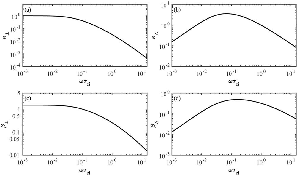
Fig. 1. Dependence of transport coefficients (a) κ_⊥, (b) κ_∧, (c) β_⊥, and (d) β_∧ on the Hall coefficient ωτ_ei.

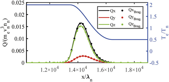
Fig. 2. Heat transport in a plasma for a temperature gradient λ_e/L_T ∼ 5 × 10⁻⁵ in a magnetic field B = B_xe_x + B_ze_z, with eB_xτ_n/m_e = ω_xτ_n = 0.1 and eB_zτ_n/m_e = ω_zτ_n = 0.1, where the heat fluxes along the x, y, and z directions obtained from the simulation (dots) are compared with those from Braginskii’s local theory (solid lines), and the temperature profile is shown by the blue line.

Fig. 3. Heat flux distributions in the absence and presence of a magnetic field B = B_ze_z. (a) and (b) Heat flux components Q_x and Q_y along the x and y directions, respectively, for a moderately large temperature gradient λ_e/L_T ≈ 0.01 at t = 200τ_n (the time at which the heat wave front roughly reaches the boundary). (c) and (d) Heat flux components Q_x and Q_y, respectively, for an extremely large temperature gradient λ_e/L_T ≈ 0.05 at t = 20τ_n. The blue solid line shows the initial temperature profile. The VFP simulation results are shown by the solid lines with ω_zτ_n = 0.05 (red) or ω_zτ_n = 0 (black), and the dotted lines are calculated from Eq. (9) with ω_zτ_n = 0.05 (red) or ω_zτ_n = 0 (black), where the instantaneous density and temperature profiles obtained from the VFP simulations are employed. Note that Q_y = 0 in the case B_z = 0.

Fig. 4. Heat flux distributions with a purely transverse magnetic field B_z or a magnetic field B = B_xe_x + B_ze_z at t = 20τ_n. (a)–(c) Heat flux components Q_x, Q_y, and Q_z, respectively, for a temperature gradient λ_e/L_T ≈ 0.05. The green lines are for ω_xτ_n = 0.1 and ω_zτ_n = 0.1, and the red lines are for ω_xτ_n = 0 and ω_zτ_n = 0.1, with the solid lines being from the simulation and the dotted lines from the Braginskii theory.

Fig. 5. Dependence of the time-averaged ratio QVFP/QBrag of the heat flux obtained from the VFP simulation to that estimated by the Braginskii theory within the first 100 collision cycles at x_max/2, where λ_e/L_T ≈ 0.05 and the distribution function is calculated up to harmonic order ℓ = 8. Different lines correspond to different strengths of the transverse magnetic field component B_z, and the dotted line in (a) corresponds to the heat flux in the absence of a magnetic field.

Fig. 6. Time evolution of the heat flux components Q_x, Q_y, and Q_z and the instantaneous scale length of the temperature gradient L_T at the point x_max/2. The initial scale length of the temperature gradient and the applied magnetic field B = B_xe_x + B_ze_z are the same as the parameters in Fig. 4. The solid lines show the heat flux in the x (black), y (red), and z (green) directions, while the dotted line represents the instantaneous scale length of the temperature gradient. The simulation is carried out with a spherical harmonic expansion up to order ℓ = 8.

Fig. 7. Ratios of the higher-order spherical harmonic terms f10, f20, f30, and f40 to the zeroth-order (isotropic) term f00 of the EDF at longitudinal positions (a) x = x_max/3, (b) x = x_max/2, and (c) x = 2x_max/3.

Fig. 8. (a)–(c) Time evolution of the heat flux components Q_x, Q_y, and Q_z, respectively, at the point x = x_max/2, where the comparison is made for different orders of the spherical harmonic expansion under a temperature gradient λ_e/L_T ≈ 0.05 and a magnetic field B = B_xe_x + B_ze_z, with eB_xτ_n/m_e = ω_xτ_n = 0.1 and eB_zτ_n/m_e = ω_zτ_n = 0.1.

Fig. 9. (a)–(c) Heat flux distributions Q_x, Q_y, and Q_z, respectively, at t = 20τ_n. The plasma and the magnetic field parameters are as in Fig. 8. The black lines and red lines are obtained with the first and ℓ = 8 spherical harmonic expansion orders, respectively, and the dotted line is the result from the Braginskii theory.