Nonlocal thermal transport in magnetized plasma along different directions

Hanzhi Zhao; Zhengming Sheng; Suming Weng

doi:10.1063/5.0086783

Abstract

Nonlocal thermal transport in magnetized plasmas is studied theoretically and numerically with the Vlasov–Fokker–Planck (VFP) model, in which the magnetic field has nonzero components both perpendicular to and along the temperature gradient. Nonlocal heat transport is found in both the longitudinal and transverse directions, provided the temperature gradients are sufficiently large. The magnetic field tends to reduce the nonlocality of the thermal transport in the direction perpendicular to the magnetic field, i.e., the difference between the heat fluxes predicted by the Braginskii theory and the VFP simulation decreases with increasing magnetic field strength. When the initial temperature gradient is steep, the nonlocal heat flux depends not only on the present temperature profile, but also on its time history. Moreover, the contribution of high-order terms in the spherical harmonic expansion of the electron distribution function becomes important for a magnetized plasma, in particular for thermal transport in the direction perpendicular to the temperature gradient.

I. INTRODUCTION

Thermal transport plays a critical role in inertial confinement fusion (ICF), leading to fusion target compression and heating. Classically, heat transport in a plasma is described by Spitzer–Härm theory.1 Assuming that the plasma is sufficiently close to thermal equilibrium, the transport coefficients can be derived by linearization of the Vlasov–Fokker–Planck (VFP) equation. However, Spitzer–Härm theory often becomes invalid in the presence of steep temperature gradients in laser-produced plasmas, where nonlocal transport models are required.2–12 Nonlocal thermal transport is also widely encountered in other plasma systems, such as magnetic fusion devices, astrophysical environments, and general laser–plasma interactions.13–24

On the other hand, megagauss magnetic fields can be self-generated in laser-produced plasmas via various mechanisms such as the Biermann battery effect when the temperature and density gradients are noncollinear,25 the Weibel instability due to anisotropic electron velocity distributions,26 and the transport of hot electrons.27 Also, it has been proposed that the application of strong external magnetic fields could improve energy coupling efficiency in ICF, and there have been some experimental implementations of this proposal.28–30 In a magnetized plasma, the transport coefficients are expressed in tensor form and are classically given by the Braginskii theory.31 On the basis of this theory, some more accurate and practical models for arbitrary atomic numbers have been proposed.32,33 Generally, magnetic fields tend to inhibit and divert the heat flux, and nonlocal thermal transport also takes place in magnetized plasmas with steep temperature gradients. In previous studies, the magnetic fields have usually been assumed to be applied in the direction perpendicular to the temperature gradient.10,11,34–37 In real experiments, however, magnetic fields can be found in arbitrary directions.

In this paper, nonlocal electron thermal transport with DC magnetic fields applied in arbitrary directions is investigated theoretically and numerically using a VFP simulation code developed with a spherical harmonics expansion method. In contrast to local heat transport, it is found that the presence of a magnetic field component along the temperature gradient can lead to significant coupling of thermal transport along the directions parallel (longitudinal) and perpendicular (transverse) to the temperature gradient in nonlocal heat transport. The remainder of the paper is structured as follows. In Sec. II, the local theory of thermal transport in a magnetized plasma is reviewed briefly. Section III introduces the basic equations and numerical scheme for the VFP code that is developed here and used in the subsequent investigation. Thermal transport in a magnetized plasma under different configurations is investigated in Sec. IV. Conclusions are presented in Sec. V.

II. THEORY OF LOCAL THERMAL TRANSPORT IN A MAGNETIZED PLASMA

Thermal transport in a fully ionized plasma can be described by the VFP equation $\frac{\partial f}{\partial t} + v \cdot \nabla f - (\frac{e E}{m_{e}} + v \times \frac{e B}{m_{e} c}) \cdot \nabla_{v} f = C_{e e} + C_{e i},$ (1)where f(v, x, t) is the electron distribution function (EDF), m_e and e are the electron mass and charge, and E and B are the electric and magnetic fields. The operators on the right-hand side represent the effects of electron–electron and electron–ion collisions. Under the assumption that the temperature gradient is sufficiently small, with ∇T_e/T_e ≪ 1/λ_e, where λ_e is the electron mean free path, the distribution function can be expanded as a homogeneous zeroth-order term plus a small anisotropic term:31 $f (v, x, t) ≃ f_{0} (v, x, t) + \frac{v}{v} \cdot f_{1} (v, x, t),$ (2)where the isotropic term f₀(v, x, t) is initially assumed to be a Maxwellian distribution given by $f_{0} = n_{e} {(m_{e} / 2 π T_{e})}^{3 / 2} \exp (- m_{e} v^{2} / 2 T_{e})$ and the perturbed term f₁(v, x, t) is related to the thermal transport due to the temperature gradient. Substituting Eq. (2) into Eq. (1), the perturbed term for the steady state can be obtained as $v \nabla f_{0} - \frac{e E}{m_{e}} \nabla_{v} f_{0} - \frac{e B}{m_{e} c} \times f_{1} = - ν_{e i} f_{1},$ (3)where ν_ei is the electron–ion collision frequency. The electron–electron collision term that would otherwise appear on the right-side of Eq. (3) can be neglected in the Lorentz gas approximation in the high-Z limit, which is valid since the characteristic electron–electron collision frequency ν_ee ≈ ν_ei/Z in neutral plasmas.31

In classical local transport models, it is usually assumed that the magnetic field B is perpendicular to the temperature gradient, because the magnetic field does not change the transport along the magnetic field for the first order of perturbations.32 Under a transverse magnetic field, the solution to Eq. (3) is given straightforwardly by $\begin{align} f_{1} = \frac{1}{ν_{e i}^{2} + ω^{2}} (- ν_{e i} g - ω \times g), \end{align}$ (4) $\begin{align} g = v \nabla f_{0} - \frac{e E}{m_{e}} \nabla_{v} f_{0}, \end{align}$ (5)where ω = eB/m_ec is the gyrofrequency of electrons in the magnetic field. Equation (4) shows that there are two terms contributing to the perturbation of the distribution function, the first of which is due to the temperature gradient and the second to the presence of the magnetic field.34 It should be noted that f₁ is rotated by the Lorentz force, and so the heat flux is no longer parallel to the temperature gradient. In addition, the “effective” electron collision frequency is reduced by the magnetic field via the factor $1 / (1 + ω^{2} / ν_{e i}^{2})$ .36

To calculate the electric field and heat flux, Eq. (4) is substituted into the Ampère–Maxwell law: $J = - \frac{4 π e}{3} \int f_{1} v^{3} d v = \frac{c}{4 π} \nabla \times B .$ (6)The heat flux is then given by $\begin{align} Q & = \frac{2 π m_{e}}{3} \int f_{1} v^{5} d v = \frac{2 π m_{e}}{3} \int \frac{v^{5}}{ν_{e i}^{2} + ω^{2}} (- ν_{e i} g - ω \times g) d v . \end{align}$ (7)In the notation adopted by Braginskii,31 the above integrations yield the following transport relations: $\begin{align} e n_{e} E = & - \nabla P_{e} + J \times B / c + α_{⊥} J / n_{e} - α_{\land} b \times J / n_{e} \\ - β_{⊥} \nabla T_{e} - β_{\land} b \times \nabla T_{e}, \end{align}$ (8) $\begin{align} Q = - (β_{⊥} + \frac{5}{2}) \frac{T_{e}}{e} J - β_{\land} \frac{T_{e}}{e} b \times J - κ_{⊥} \nabla T_{e} - κ_{\land} b \times \nabla T_{e}, \end{align}$ (9)where P_e is the scalar intrinsic pressure, n_e is the electron number density, and b is the unit vector in the magnetic field direction. The κ coefficients are for the thermal heat flux from temperature gradients, whereas the β coefficients give the heat flux driven by electric currents. These quantities are expressed in terms of components parallel to the driving terms, which are perpendicular to the magnetic field and indicated by subscript ⊥, and components in a crossed direction, which are perpendicular to both the magnetic field and the driving term and indicated by subscript ∧. The driving terms are the current density and temperature gradient. The transport coefficients read as follows:35 $\begin{array}{c} κ_{⊥} = \frac{2 T_{e} n_{e}}{m_{e} v_{T}} |Ω| \frac{ϕ_{11} ϕ_{7}^{2} - ϕ_{7} ϕ_{9}^{2} + Ω^{2} (ϕ_{11} ϕ_{10}^{2} + ϕ_{7} ϕ_{12}^{2} - 2 ϕ_{9} ϕ_{10} ϕ_{12})}{ϕ_{7}^{2} + Ω^{2} ϕ_{10}^{2}}, \\ κ_{\land} = \frac{2 T_{e} n_{e}}{m_{e} v_{T}} \frac{ϕ_{14} ϕ_{7}^{2} + ϕ_{10} ϕ_{9}^{2} + 2 ϕ_{7} ϕ_{9} ϕ_{12} + Ω^{2} (ϕ_{14} ϕ_{10}^{2} - ϕ_{10} ϕ_{12}^{2})}{ϕ_{7}^{2} + Ω^{2} ϕ_{10}^{2}}, \\ β_{⊥} = |Ω| \frac{ϕ_{9} ϕ_{7} + Ω^{2} ϕ_{12} ϕ_{10}}{ϕ_{7}^{2} + Ω^{2} ϕ_{10}^{2}} - \frac{5}{2}, β_{\land} = \frac{ϕ_{12} ϕ_{7} - ϕ_{9} ϕ_{10}}{ϕ_{7}^{2} + Ω^{2} ϕ_{10}^{2}}, \\ α_{⊥} = \frac{1}{2} m_{e} n_{e} v_{T} \frac{ϕ_{7}}{ϕ_{7}^{2} + Ω^{2} ϕ_{10}^{2}}, \\ α_{\land} = \frac{1}{2} m_{e} n_{e} v_{T} |Ω| (1 - \frac{ϕ_{10}}{ϕ_{7}^{2} + Ω^{2} ϕ_{10}^{2}}), \end{array}$ (10)where Ω = ωτ_ei is the Hall coefficient, τ_ei is the electron–ion collision time, u = v/v_te is the normalized velocity with $v_{t e} = \sqrt{2 T_{e} / m_{e}}$ , and the dimensionless functions ϕ_n are $ϕ_{n} (Ω) = \frac{4}{3 \sqrt{π}} \int \frac{u^{n} e^{- u^{2}} d u}{1 + Ω^{2} u^{6}} .$ (11)

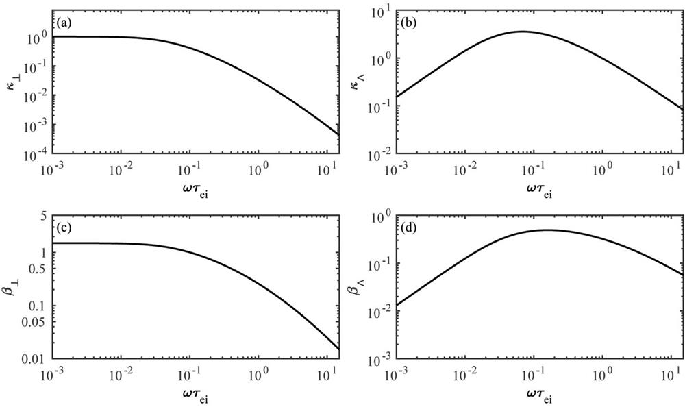
Figure 1 shows the transport coefficients as functions of the applied magnetic field strength ωτ_ei, which indicates both the suppression and deflection of the heat flux by the magnetic field. As the magnetic field increases, the transport coefficients κ_⊥ and β_⊥ along the temperature gradient decay rapidly, while the crossed transport coefficients κ_∧ and β_∧ perpendicular to the gradient and the magnetic field first increase before ωτ_ei ∼ 0.1 and then decrease.

Figure 1.Dependence of transport coefficients (a) κ_⊥, (b) κ_∧, (c) β_⊥, and (d) β_∧ on the Hall coefficient ωτ_ei.

III. DEVELOPMENT OF THE VFP CODE

Since the diffusion approximation is used, the above theory is limited to local thermal transport. To study nonlocal thermal transport under magnetic fields along arbitrary directions, we have developed a VFP code with a longitudinal spatial coordinate and three velocity components (1D3V) for electrons, while the ions are fixed as a neutral background. Generally, the VFP equation can be written as $\frac{\partial f}{\partial t} + v_{x} \frac{\partial f}{\partial x} - (\frac{e E}{m_{e}} + v \times \frac{e B}{m_{e} c}) \cdot \nabla_{v} f = C_{e e} + C_{e i} .$ (12)

Even though the VFP equation gives a complete description of electron dynamics, direct solution of this equation is difficult. An efficient way is to reduce the computational cost by expanding the distribution function in spherical harmonics $Y_{ℓ}^{m}$ , with the expansion being truncated at a certain order ℓ:38–40 $f (v, x, t) = \sum_{ℓ = 0}^{\infty} \sum_{m = - ℓ}^{ℓ} f_{ℓ}^{m} (v, x, t) Y_{ℓ}^{m} .$ (13)

This approach is acceptable because the collisions ensure that the distribution function tends to isotropy. On substitution of the above expansion into Eq. (12), the equation for the harmonic components can be written as $\frac{\partial f_{ℓ}^{m}}{\partial t} {+ A}_{ℓ}^{m} {+ E}_{ℓ}^{m} {+ B}_{ℓ}^{m} {= C}_{ℓ}^{m} .$ (14)On the left-hand side of Eq. (14), $A_{ℓ}^{m}$ represents the contribution of spatial advection, $E_{ℓ}^{m}$ that of electric fields, and $B_{ℓ}^{m}$ that of magnetic fields, while the term on the right-hand side is due to collisions (see Ref. 39 for more details of the terms on both sides). The electric field is calculated via the quasineutral approximation or by Ampère’s law, and we ignore the evolution of the magnetic fields. The timescale of electron transport is much shorter than that of ion motion, and so the ions are treated as a cold background.

The numerical implementations for solving the equations are identical to the methods in Ref. 40. The central difference approach is used for the derivatives in real space, and the Vlasov operator on the left-hand side is integrated by the Runge–Kutta method. Following the Chang–Cooper scheme,41 the Fokker–Planck collision operator is differenced using an implicit and energy-conserving scheme according to Ref. 42.

To simplify the study, we normalize the variables as follows: $\begin{aligned} v & \to \frac{v}{v_{n}}, & t & \to \frac{t}{τ_{n}}, & x & \to \frac{x}{λ_{n}}, \\ f & \to \frac{v_{n}^{3} f}{n_{n}}, & E & \to \frac{e τ_{n}^{2} E}{m_{e} λ_{n}}, & B & \to \frac{e B τ_{n}}{m_{e}}, \end{aligned}$ (15)where the temperature is normalized to a reference value T_n and the density to n_n. Correspondingly, $v_{n} = \sqrt{2 k_{B} T_{n} / m_{e}}$ is the thermal velocity, $τ_{n} = m_{e}^{2} v_{n}^{3} / (4 π Z e^{4} n_{n} \ln Λ)$ is the electron–ion collision time, and λ_n = v_nτ_n. For simplicity, the Coulomb logarithm ln Λ is assumed to be constant everywhere in spatial space.

To validate the code, we have carried out benchmark studies by comparing the simulation results with those of the classical local transport theory given in Sec. II. The initial temperature profile is $T_{e} (x) = \{\begin{cases} T_{0}, & x > 2 x_{\max} / 3, \\ T_{0} + 2 Δ T, & x < x_{\max} / 3, \\ T_{0} + Δ T - Δ T \cos (\frac{3 x}{x_{\max}} π), & e l s e w h e r e . \end{cases}$ (16)

By varying the values of x_max and ΔT, different temperature gradients can be obtained. The magnetic field is uniform, and so J = 0 and the heat flux driven by the current is zero. The plasma is initialized under the assumptions that the density is spatially uniform, the electron distribution is Maxwellian, and Z = 16. A continuous boundary condition is applied on two boundaries along the x direction. The simulation is stopped when the heat wave front reaches the boundary.

In the case of an unmagnetized plasma, according to the local transport theory, the electrons with velocities near v ≃ 3.7v_te make the greatest contribution to the heat flux. Correspondingly, f₁ ≈ 533(λ_e/L_T)f_M at v ≃ 3.7v_te, where L_T = T_e/∇T_e is the scale length. Therefore, the classical electron thermal transport theory only holds when λ_e/L_T ≪ 10⁻³. We have carried out a numerical simulation in the local transport regime. Figure 2 presents the heat transport along the temperature gradient with ΔT = 1.5T₀, where the degree of nonlocality at x = x_max/2 is about λ_e/L_T ∼ 5 × 10⁻⁵, and the magnetic field B = B_xe_x + B_ze_z, with eB_xτ_n/m_e = ω_xτ_n = 0.1 and eB_zτ_n/m_e = ω_zτ_n = 0.1. It is confirmed that the simulation results obtained with our code agree well with those of the local transport theory. It is worth mentioning that the Braginskii heat fluxes are calculated using the instantaneous density and temperature profiles obtained from the VFP simulations.

Figure 2.Heat transport in a plasma for a temperature gradient λ_e/L_T ∼ 5 × 10⁻⁵ in a magnetic field B = B_xe_x + B_ze_z, with eB_xτ_n/m_e = ω_xτ_n = 0.1 and eB_zτ_n/m_e = ω_zτ_n = 0.1, where the heat fluxes along the x, y, and z directions obtained from the simulation (dots) are compared with those from Braginskii’s local theory (solid lines), and the temperature profile is shown by the blue line.

IV. SIMULATIONS OF NONLOCAL TRANSPORT IN MAGNETIZED PLASMAS

A. Nonlocal transport under magnetic fields along different directions

Using the VFP code, we investigate the coupling of thermal transports along the directions parallel and perpendicular to the temperature gradient in the presence of a DC magnetic field along different directions.

First, we consider a magnetic field applied along the transverse (z) direction, which will lead to thermal transport in the y direction besides the transport along the temperature gradient in the x direction. When the condition λ_e/L_T ≪ 10⁻³ is not satisfied, the electron distribution function (EDF) will no longer be Maxwellian. Furthermore, the perturbation f₁ may be greater than f₀ in some velocity region, which will cause breakdown of the local theory of thermal transport. As a result, the heat flux calculated by the classical theoretical models will be significantly overestimated in the case of a large temperature gradient. Figure 3 shows the heat flux along the directions parallel and perpendicular to a large temperature gradient. At a moderately large temperature gradient λ_e/L_T ≈ 0.01, Fig. 3(a) clearly shows that nonlocal transport appears in an unmagnetized plasma. Our VFP simulation demonstrates that the peak heat flux Q_x with B_z = 0 is much smaller than the saturated heat flux predicted by Spitzer–Härm theory. Moreover, the heat flux obtained from our VFP simulation is distributed over a wider area, which implies the existence of a preheating effect due to the nonlocal thermal transport.

Figure 3.Heat flux distributions in the absence and presence of a magnetic field B = B_ze_z. (a) and (b) Heat flux components Q_x and Q_y along the x and y directions, respectively, for a moderately large temperature gradient λ_e/L_T ≈ 0.01 at t = 200τ_n (the time at which the heat wave front roughly reaches the boundary). (c) and (d) Heat flux components Q_x and Q_y, respectively, for an extremely large temperature gradient λ_e/L_T ≈ 0.05 at t = 20τ_n. The blue solid line shows the initial temperature profile. The VFP simulation results are shown by the solid lines with ω_zτ_n = 0.05 (red) or ω_zτ_n = 0 (black), and the dotted lines are calculated from Eq. (9) with ω_zτ_n = 0.05 (red) or ω_zτ_n = 0 (black), where the instantaneous density and temperature profiles obtained from the VFP simulations are employed. Note that Q_y = 0 in the case B_z = 0.

When a transverse magnetic field is applied along the z direction with a normalized field strength ω_zτ_n = 0.05, which is about 16 T for a plasma with Z = 16, n_e = 10²¹ cm⁻³, and T_e = 2.5 keV. It is found that the heat flux Q_x along the temperature gradient can be significantly reduced in comparison with the unmagnetized case. In the case ω_zτ_n = 0.05, the heat flux Q_x obtained from the VFP simulation almost coincides with that estimated by the classical Braginskii model, indicating that thermal transport with a large temperature gradient may become local again under a strong transverse magnetic field. However, Fig. 3(b) shows that a transverse heat flux Q_y along the y direction will be present in the case of a transverse magnetic field B_z. As illustrated in Fig. 3(b), this transverse heat flux Q_y is well predicted by the Braginskii theory for a moderately large temperature gradient λ_e/L_T ≈ 0.01. This is because the magnetic field will be able to localize the heat flux if the Larmor radius is much shorter than the scale length of the temperature gradient.36 For the magnetic field ωτ_n = 0.05 and temperature gradient λ_e/L_T ≃ 0.01 used in Fig. 3(b), we have r_L/L_T ≈ 0.2.

For comparison, Figs. 3(c) and 3(d) show the heat flux with a large temperature gradient λ_e/L_T ≈ 0.05. In this case, nonlocal transport becomes significant for both the unmagnetized and magnetized plasmas. More importantly, the nonlocal thermal transport in this case occurs not only along the temperature gradient (Q_x) but also along the transverse direction (Q_y) with B_z ≠ 0. The thermal transport along the y direction exhibits a stronger nonlocality than that along the x direction. Usually, the so-called heat flux limiter $|Q_{VFP} / m_{e} n_{e} v_{t e}^{3}|$ can be used to estimate the degree of nonlinearity of the transport, and a flux limiter of 0.15 is often used in MHD fluid codes.43,44 The limiter is around 0.7 for the longitudinal heat flux in Fig. 3(c), while for the Righi–Leduc heat flux in Fig. 3(d) it is about 0.18. That is to say, the VFP simulations show that the heat flux limiter for the transverse (Righi–Leduc) heat flux is much smaller than that for the standard component of the longitudinal heat flux.

We now consider the case in which the DC magnetic field has nonzero components along both the transverse (z) and longitudinal (x) directions: B = B_xe_x + B_ze_z. The thermal flux Q_z along the z direction is now no longer zero, since the magnetic field B_x along the x direction can divert the heat flux Q_y along the y direction to the z direction. According to the local heat transport theory, the transport parallel to the magnetic field will not be affected by the applied magnetic field. Taking the scalar product of both sides of Eq. (3) with B gives B · [v∇f₀ − (eE/m_e)∇_vf₀ + ν_eif₁] = 0. Therefore, without loss of generality, it can be assumed that the magnetic field is perpendicular to the heat flux, i.e., f₁ · ω = 0. In the nonlocal transport regime, however, the isotropic part of the electron distribution can be far from Maxwellian, and its evolution is associated with all the components of f₁. Furthermore, the first-order expansion is no longer sufficiently accurate in the nonlocal transport regime. Actually, high-order spherical harmonic terms play an important role in the transport process, and the first-order harmonic f₁ is strongly coupled with those high-order terms, as shown in the following.

Figure 4 compares the heat fluxes along different directions with a large temperature gradient λ_e/L_T ≈ 0.05 under a magnetic field B = B_xe_x + B_ze_z. We truncate the spherical harmonic expansion at order ℓ = 8 here. Figure 4(a) shows that in comparison with the case of a purely transverse magnetic field B = B_ze_z, the heat flux Q_x along the temperature gradient can be slightly enhanced by the x component of the magnetic field B = B_xe_x + B_ze_z, and the Braginskii theory significantly overestimates Q_x. By contrast, Fig. 4(b) shows that the heat flux Q_y along the cross direction will be significantly reduced by the B_x component of the magnetic field. This is because B_x will deflect the heat flux Q_y partially into the heat flux Q_z. As another consequence, a nonzero Q_z is induced, as shown in Fig. 4(c). As can be seen from Figs. 4(b) and 4(c), the Braginskii theory significantly overestimates Q_y as well as Q_z.

Figure 4.Heat flux distributions with a purely transverse magnetic field B_z or a magnetic field B = B_xe_x + B_ze_z at t = 20τ_n. (a)–(c) Heat flux components Q_x, Q_y, and Q_z, respectively, for a temperature gradient λ_e/L_T ≈ 0.05. The green lines are for ω_xτ_n = 0.1 and ω_zτ_n = 0.1, and the red lines are for ω_xτ_n = 0 and ω_zτ_n = 0.1, with the solid lines being from the simulation and the dotted lines from the Braginskii theory.

In Fig. 5, we plot the time-averaged ratio $|Q_{VFP} / Q_{Brag}|$ of the heat flux obtained from the VFP simulation to that estimated by the Braginskii theory under different magnetic fields at x_max/2. When the magnetic field is perpendicular to the temperature gradient (ω_xτ_n = 0), the transverse magnetic field B_z inhibits the nonlocal effect, and the heat flux in the x direction is almost local when ω_zτ_n ≥ 0.1. The heat flux Q_y in the y direction from the VFP simulation is significantly smaller than that estimated by the Braginskii theory, and the radio $|Q_{VFP} / Q_{Brag}|$ is always smaller than 0.4 for ω_zτ_n ≤ 0.125. This indicates that the transverse magnetic field B_z can localize the heat flux Q_x along the temperature gradient with ω_xτ_n ≥ 0.1 (the corresponding r_L/L_T ≤ 0.05). However, this transverse magnetic field will induce a nonzero heat flux Q_y in the y direction, and the classical Braginskii theory will overestimate the value of Q_y. The heat fluxes Q_y and Q_z in the two transverse directions can be localized by an increase in the magnetic field component B_x along the temperature gradient, as shown in Figs. 5(b) and 5(c), since electron transverse motion will be suppressed by the longitudinal magnetic field B_x, thereby reducing the effective electron mean free path in the transverse directions.34 However, Fig. 5(a) shows that the Braginskii theory overestimates the heat flux Q_x more with increasing B_x, and the heat transport along the temperature gradient exhibits a stronger nonlocality. With the increase of the longitudinal magnetic field B_x, the electrons will be guided along the x direction and the transverse electron motion will be suppressed. Consequently, the heat flux Q_x is enhanced, while the heat fluxes Q_y and Q_z in the transverse directions are localized. Therefore, with increasing B_x, the heat transport along the x direction exhibits a stronger nonlocality with a smaller Q_x,VFP/Q_x,Brag, as shown in Fig. 5(a). In the NIF, the typical L_T is about 5 mm,45,46 and so magnetic fields of the order of several tesla are high enough to affect the transport process. The experiment also shows that an external field along the hohlraum results in a significant increase in plasma temperature.47

Figure 5.Dependence of the time-averaged ratio $|Q_{VFP} / Q_{Brag}|$ of the heat flux obtained from the VFP simulation to that estimated by the Braginskii theory within the first 100 collision cycles at x_max/2, where λ_e/L_T ≈ 0.05 and the distribution function is calculated up to harmonic order ℓ = 8. Different lines correspond to different strengths of the transverse magnetic field component B_z, and the dotted line in (a) corresponds to the heat flux in the absence of a magnetic field.

As shown in Fig. 4(c), a nonzero Q_z will be induced owing to the rotation of Q_y by the B_x component of the magnetic field. Figure 5(c) further shows that the Q_z obtained from the VFP simulations is always much lower than that estimated by the classical Braginskii theory $(|Q_{z, V F P} / Q_{z, B r a g}| \leq 0.1)$ . That is to say, the nonlocality of the heat flux component Q_z is more significant, and hence Q_z should be treated more carefully.

In our simulations, the initial electron distribution function is assumed to be Maxwellian, and therefore a certain response time is required to generate the heat flux. In the local transport theory, the Braginskii transport is a quasistatic state. When the temperature gradient is steep, however, we find that the heat flux cannot reach a quasistatic value before the temperature profile changes significantly. For an initial steep temperature gradient λ_e/L_T ≈ 0.05, Fig. 6 shows that the growth rates of the heat flux components along different directions are significantly different. The heat flux Q_x in the x direction increases most rapidly at the beginning, reaching a peak at t ∼ 5τ_n. It then decays rapidly during 5τ_n ≤ t ≤ 20τ_n and slowly after t ∼ 30τ_n. In comparison, the growth rates of the heat flux components in the y and z directions are slower. The heat flux Q_x is due mainly to the temperature gradient along the x direction, while the heat flux components Q_y and Q_z in the directions perpendicular to the temperature gradient come from deflection by the magnetic field, which naturally lags behind the growth of Q_x. The result is that the nonlocal heat flux depends not only on the current temperature profile, but also on the history of the temperature profile. This could be one reason why some nonlocal heat flux models fail, since they only consider the T_e profile at the current time.

Figure 6.Time evolution of the heat flux components Q_x, Q_y, and Q_z and the instantaneous scale length of the temperature gradient L_T at the point x_max/2. The initial scale length of the temperature gradient and the applied magnetic field B = B_xe_x + B_ze_z are the same as the parameters in Fig. 4. The solid lines show the heat flux in the x (black), y (red), and z (green) directions, while the dotted line represents the instantaneous scale length of the temperature gradient. The simulation is carried out with a spherical harmonic expansion up to order ℓ = 8.

B. Effects of harmonic expansion order

In the local transport theory, the diffusion approximation is usually adopted, with only the first-order spherical harmonic being considered. However, the situation is much more complicated in the nonlocal transport regime, particularly in magnetized plasmas, where transverse thermal transport is induced as well. Figure 7 shows the ratios of the higher-order spherical harmonic terms $f_{1}^{0}$ , $f_{2}^{0}$ , $f_{3}^{0}$ , and $f_{4}^{0}$ to the zeroth-order (isotropic) term $f_{0}^{0}$ of the EDF in velocity space at the points x = x_max/3, x_max/2, and 2x_max/3 in the nonlocal regime. For a relatively large temperature gradient, it can be seen that the first-order term $f_{1}^{0}$ can be greater than the isotropic term $f_{0}^{0}$ in the high-energy region around v ≈ 3.7v_n that makes the greatest contribution to the heat flux. Also, the high-order terms appear to be more important in the spatial region around x = 2x_max/3 where the relatively cold plasma is preheated by the electrons at the tail of the electron distribution function. By contrast, the high-order terms are not so important at the top of the temperature profile (x ≤ x_max/3). In particular, the high-order spherical harmonic terms can become comparable to or even larger than the zeroth-order term $f_{0}^{0}$ in the high-energy velocity region. Therefore, linear perturbation theory is no longer valid, and the contributions of those high-order terms must be considered precisely in the nonlocal transport model.

Figure 7.Ratios of the higher-order spherical harmonic terms $f_{1}^{0}$ , $f_{2}^{0}$ , $f_{3}^{0}$ , and $f_{4}^{0}$ to the zeroth-order (isotropic) term $f_{0}^{0}$ of the EDF at longitudinal positions (a) x = x_max/3, (b) x = x_max/2, and (c) x = 2x_max/3.

Considering higher-order expansion terms, the components of $f_{1}^{0}$ and $f_{1}^{1}$ will be coupled together through $f_{2}^{m}$ (for m = 0, 1, 2). Therefore, the magnetic field component B_x along the temperature gradient will also affect the transport process. Figure 8 shows the time evolution of the heat flux at the point x = x_max/2 when the magnetic field is not completely perpendicular to the temperature gradient. As can be seen, the truncated order of the spherical harmonic expansion used in the VFP simulation has a relatively weak effect on the heat flux Q_x in the x direction, but a more significant effect on the heat fluxes Q_y and Q_z. With the first-order expansion term only, all the components Q_x, Q_y, and Q_z of the heat flux are overestimated, while with the first two expansion terms, all the components are underestimated. More interestingly, the higher-order terms have a more significant effect on the heat flux components Q_y and Q_z that are perpendicular to the temperature gradient. Generally, we find that the VFP simulation results converge when the expansion is taken up to order ℓ = 8, as has been done in the simulations presented above.

Figure 8.(a)–(c) Time evolution of the heat flux components Q_x, Q_y, and Q_z, respectively, at the point x = x_max/2, where the comparison is made for different orders of the spherical harmonic expansion under a temperature gradient λ_e/L_T ≈ 0.05 and a magnetic field B = B_xe_x + B_ze_z, with eB_xτ_n/m_e = ω_xτ_n = 0.1 and eB_zτ_n/m_e = ω_zτ_n = 0.1.

The effect of high-order terms on the distribution of the heat flux is shown in Fig. 9. It is found that the strong preheating effect at the heat front of Q_y and Q_z can be exactly preserved only when the high-order spherical harmonic terms are retained, while the first-order spherical harmonic expansion is already enough to treat the preheating effect at the heat front of Q_x.

Figure 9.(a)–(c) Heat flux distributions Q_x, Q_y, and Q_z, respectively, at t = 20τ_n. The plasma and the magnetic field parameters are as in Fig. 8. The black lines and red lines are obtained with the first and ℓ = 8 spherical harmonic expansion orders, respectively, and the dotted line is the result from the Braginskii theory.

V. CONCLUSIONS

The nonlocal thermal transport process in magnetized plasmas has been studied theoretically and numerically with the VFP model, in which the magnetic field has nonzero components both perpendicular to and along the temperature gradient. For this purpose, a VFP code with one-dimensional spatial coordinate and three-dimensional velocity components has been developed. Generally, the magnetic field component perpendicular to the temperature gradient tends to restrain the heat flux along this gradient and induces a transverse heat flux. When the magnetic field has two components along the transverse and longitudinal directions, it is found that the heat flux along the third direction appears via a coupling between the longitudinal magnetic field and the transverse heat flux. Nonlocal heat transport is found in both the longitudinal and transverse directions, provided the temperature gradients are sufficiently large. For nonlocal transport under a magnetic field along an arbitrary direction, the magnetic field will reduce the nonlocality of the heat transport in the direction perpendicular to the magnetic field, i.e., the difference between the heat fluxes predicted by the Braginskii theory and the VFP simulations tends to decrease with increasing magnetic field strength. In real experiments, transverse magnetic fields are induced at laser ablation fronts. We note that external magnetic fields are now being introduced on purpose to control plasma temperature and density profiles.48–50 Generally, a transverse heat flux may be beneficial to the formation of a more uniform ablation front with a higher temperature.51 Furthermore, a stronger nonlocal effect in the transverse direction can reduce heat transport and produce plasmas with different geometrical features, and so it is important to implement an appropriate thermal transport model in MHD simulations.

More importantly, the nonlocal heat flux depends not only on the current but also on the preceding temperature profiles. In the process of heat flux evolution, the response time of the heat flux component along the temperature gradient is much shorter than that of the component perpendicular to the gradient. When the temperature gradient is steep, the contribution of higher-order terms in the spherical harmonic expansion of the electron distribution function becomes important even for weakly magnetized plasmas, especially for the thermal transport in the direction perpendicular to the temperature gradient.

ACKNOWLEDGMENTS

Acknowledgment. This work is supported by the Strategic Priority Research Program of the Chinese Academy of Sciences (Grant No. XDA25050100), the National Natural Science Foundation of China (Grant Nos. 12135009 and 11975154), and the Science Challenge (Project No. TZ2018005).

References

[1] L. Spitzer, R.H?rm. Transport phenomena in a completely ionized gas. Phys. Rev., 89, 977(1953).

[2] A. R.Bell, R. G.Evans, D. J.Nicholas. Electron energy transport in steep temperature gradients in laser-produced plasmas. Phys. Rev. Lett., 46, 243(1981).

[3] D.Hull, D. R.Gray, J. D.Kilkenny, P.Blyth, M. S.White. Observation of severe heat-flux limitation and ion-acoustic turbulence in a laser-heated plasma. Phys. Rev. Lett., 39, 1270(1977).

[4] E. M.Epperlein, G. J.Rickard, A. R.Bell. Two-dimensional nonlocal electron transport in laser-produced plasmas. Phys. Rev. Lett., 61, 2453(1988).

[5] W. L.Kruer, D. E.Hinkel, D. A.Callahan, L. J.Suter, P. A.Michel, E. A.Williams, H. A.Scott, M. D.Rosen, R. P. J.Town, L.Divol et al. The role of a detailed configuration accounting (DCA) atomic physics package in explaining the energy balance in ignition-scale hohlraums. High Energy Density Phys., 7, 180-190(2011).

[6] D.Cao, G.Moses, J.Delettrez. Improved non-local electron thermal transport model for two-dimensional radiation hydrodynamics simulations. Phys. Plasmas, 22, 082308(2015).

[7] E. M.Epperlein, R. W.Short. A practical nonlocal model for electron heat transport in laser plasmas. Phys. Fluids B, 3, 3092-3098(1991).

[8] P. D.Nicola?, M.Busquet, G. P.Schurtz. A nonlocal electron conduction model for multidimensional radiation hydrodynamics codes. Phys. Plasmas, 7, 4238-4249(2000).

[9] W. Y.Huo, K.Li. Nonlocal electron heat transport under the non-Maxwellian distribution function. Phys. Plasmas, 27, 062705(2020).

[10] T. H.Kho, M. G.Haines. Nonlinear electron transport in magnetized laser plasmas. Phys. Fluids, 29, 2665-2671(1986).

[11] P.Mora, A.Bendib, J. F.Luciani. Magnetic field and nonlocal transport in laser-created plasmas. Phys. Rev. Lett., 55, 2421(1985).

[12] J. F.Luciani, P.Mora, J.Virmont. Nonlocal heat transport due to steep temperature gradients. Phys. Rev. Lett., 51, 1664(1983).

[13] R. V.Bravenec, W. L.Rowan, J.Heard, K. W.Gentle, G. A.Hallock, H.Gasquet, A.Ouroua, G.Cima, T. P.Crowley, P. E.Phillips et al. Strong nonlocal effects in a tokamak perturbative transport experiment. Phys. Rev. Lett., 74, 3620(1995).

[14] P.Galli, P.Mantica, G.Gorini, G. M. D.Hogeweij, N. J.Lopes Cardozo, J.De Kloe. Nonlocal transient transport and thermal barriers in Rijnhuizen Tokamak Project plasmas. Phys. Rev. Lett., 82, 5048(1999).

[15] B. D.Dudson, J. T.Omotani, J. P.Brodrick, M. R. K.Wigram, C. P.Ridgers. Incorporating nonlocal parallel thermal transport in 1D ITER SOL modelling. Nucl. Fusion, 60, 076008(2020).

[16] C. R.DeVore, J. T.Karpen. Nonlocal thermal transport in solar flares. Astrophys. J., 320, 904-912(1987).

[17] N. H.Bian, A. G.Emslie. Reduction of thermal conductive flux by non-local effects in the presence of turbulent scattering. Astrophys. J., 865, 67(2018).

[18] J.Büchner, M. V.Alves, S. S. A.Silva, J. C.Santos. Nonlocal heat flux effects on temperature evolution of the solar atmosphere. Astron. Astrophys., 615, A32(2018).

[19] D. M.Chambers, A.Gouveia, S. H.Glenzer, J.Hawreliak, S.Topping, P.Soundhauss, P. A.Pinto, O.Renner, R. S.Marjoribanks, R. J.Kingham et al. Thomson scattering measurements of heat flow in a laser-produced plasma. J. Phys. B: At., Mol. Opt. Phys., 37, 1541(2004).

[20] M.Edwards, P.Davis, L.Divol, R.Town, D.Froula, B.Pollock, A.Offenberger, J.Ross, D.Price, A.James et al. Quenching of the nonlocal electron heat transport by large external magnetic fields in a laser-produced plasma measured with imaging Thomson scattering. Phys. Rev. Lett., 98, 135001(2007).

[21] M.Tzoufras, A. R.Bell. Electron transport and shock ignition. Plasma Phys. Controlled Fusion, 53, 045010(2011).

[22] J.Limpouch, M.Zeman, M.Holec, J.Nikl, S.Weber, M.Kucha?ík. Macroscopic laser–plasma interaction under strong non-local transport conditions for coupled matter and radiation. Matter Radiat. Extremes, 3, 110-126(2018).

[23] J.Liu, Z.Li, Z.Yang, L.Hou, L.Guo, D.Yang, K.Lan, G.Ren, S.Li, W.Huo et al. First demonstration of improving laser propagation inside the spherical hohlraums by using the cylindrical laser entrance hole. Matter Radiat. Extremes, 1, 2-7(2016).

[24] S.Takeda, T.Johzaki, M.Horio, Y.Sentoku, M.Hino, W.Kim, S.Fujioka, A.Sunahara, T.Endo, H.Nagatomo. Intensification of laser-produced relativistic electron beam using converging magnetic fields for ignition in fast ignition laser fusion. High Energy Density Phys., 36, 100841(2020).

[25] S.Bandyopadhyay, M.Notley, P.Fernandes, M. C.Kaluza, M.Sherlock, M. S.Wei, P. M.Nilson, S.Minardi, L.Willingale, C.Kamperidis et al. Magnetic reconnection and plasma dynamics in two-beam laser-solid interactions. Phys. Rev. Lett., 97, 255001(2006).

[26] E. S.Weibel. Spontaneously growing transverse waves in a plasma due to an anisotropic velocity distribution. Phys. Rev. Lett., 2, 83(1959).

[27] A. D.Lad, W. J.Ding, Z. M.Sheng, P.Kaw, S.Ahmad, S.Mondal, S.Sengupta, V.Narayanan, B.Hao, W. M.Wang et al. Direct observation of turbulent magnetic fields in hot, dense laser produced plasmas. Proc. Natl. Acad. Sci. U. S. A., 109, 8011-8015(2012).

[28] E. C.Harding, C. E.Myers, M. R.Gomez, S. B.Hansen, S. A.Slutz, D. A.Yager-Elorriaga, D. J.Ampleford, M. R.Weis, C. A.Jennings, K. D.Hahn et al. Performance scaling in magnetized liner inertial fusion experiments. Phys. Rev. Lett., 125, 155002(2020).

[29] R. A.Vesey, S. A.Slutz. High-gain magnetized inertial fusion. Phys. Rev. Lett., 108, 025003(2012).

[30] W. M.Wang, P.Gibbon, Z. M.Sheng, Y. T.Li. Magnetically assisted fast ignition. Phys. Rev. Lett., 114, 015001(2015).

[31] S.Braginskii. Transport processes in a plasma. Rev. Plasma Phys., 1, 249-251(1965).

[32] M. G.Haines, E. M.Epperlein. Plasma transport coefficients in a magnetic field by direct numerical solution of the Fokker–Planck equation. Phys. Fluids, 29, 1029-1041(1986).

[33] H.Li, C. A.Walsh, J. D.Sadler. Symmetric set of transport coefficients for collisional magnetized plasma. Phys. Rev. Lett., 126, 075001(2021).

[34] V.Tikhonchuk, P.Nicola?, J.-L.Feugeas, M.Olazabal-Loumé, B.Dubroca, D.Del Sorbo. Extension of a reduced entropic model of electron transport to magnetized nonlocal regimes of high-energy-density plasmas. Laser Part. Beams, 34, 412-425(2016).

[35] G. P.Schurtz, J.-L. A.Feugeas, P. D.Nicola?. A practical nonlocal model for heat transport in magnetized laser plasmas. Phys. Plasmas, 13, 032701(2006).

[36] A.Nishiguchi. Nonlocal electron heat transport in magnetized dense plasmas. Plasma Fusion Res., 9, 1404096(2014).

[37] R. J.Kingham, A. G.Thomas, C. P.Ridgers. Magnetic cavitation and the reemergence of nonlocal transport in laser plasmas. Phys. Rev. Lett., 100, 075003(2008).

[38] T. W.Johnston. Cartesian tensor scalar product and spherical harmonic expansions in Boltzmann’s equation. Phys. Rev., 120, 1103(1960).

[39] W.Rozmus, A. P. L.Robinson, M.Sherlock, A. R.Bell, R. J.Kingham. Fast electron transport in laser-produced plasmas and the KALOS code for solution of the Vlasov–Fokker–Planck equation. Plasma Phys. Controlled Fusion, 48, R37(2006).

[40] M.Tzoufras, P. A.Norreys, F. S.Tsung, A. R.Bell. A Vlasov–Fokker–Planck code for high energy density physics. J. Comput. Phys., 230, 6475-6494(2011).

[41] G.Cooper, J. S.Chang. A practical difference scheme for Fokker-Planck equations. J. Comput. Phys., 6, 1-16(1970).

[42] A. R.Bell, R. J.Kingham. An implicit Vlasov–Fokker–Planck code to model non-local electron transport in 2-D with magnetic fields. J. Comput. Phys., 194, 1-34(2004).

[43] G. D.Kerbel, D. A.Liedahl, L. J.Suter, D. E.Hinkel, O. S.Jones, W. A.Farmer, J. D.Moody, D. J.Strozzi, M. A.Barrios, J. M.Koning et al. Heat transport modeling of the dot spectroscopy platform on NIF. Plasma Phys. Controlled Fusion, 60, 044009(2018).

[44] R. L.McCrory, R. C.Malone, R. L.Morse. Indications of strongly flux-limited electron thermal conduction in laser-target experiments. Phys. Rev. Lett., 34, 721(1975).

[45] L. J.Suter, J. D.Kilkenny, M. A.Barrios, W.Farmer, H.Chen, M.Sherlock, O.Jones, J. D.Moody, J.Jaquez, R. L.Kauffman et al. Developing an experimental basis for understanding transport in NIF hohlraum plasmas. Phys. Rev. Lett., 121, 095002(2018).

[46] B. J.MacGowan, S. H.Glenzer, B. H.Wilde, L. J.Suter, M. A.Blain, R. E.Turner, J. D.Lindl, G. F.Stone, C. A.Back, O. L.Landen. Thomson scattering from inertial-confinement-fusion hohlraum plasmas. Phys. Rev. Lett., 79, 1277(1997).

[47] J. R.Davies, A. B.Sefkow, B. J.Albright, P. Y.Chang, G.Fiksel, M. J.MacDonald, D. S.Montgomery, D. H.Froula, J. L.Kline, D. H.Barnak et al. Use of external magnetic fields in hohlraum plasmas to improve laser-coupling. Phys. Plasmas, 22, 010703(2015).

[48] C.Plechaty, A. A.Esaulov, R.Presura. Focusing of an explosive plasma expansion in a transverse magnetic field. Phys. Rev. Lett., 111, 185002(2013).

[49] A. V.Maximov, R.Betti, V. V.Ivanov, L. S.Leal, A. B.Sefkow. Modeling magnetic confinement of laser-generated plasma in cylindrical geometry leading to disk-shaped structures. Phys. Plasmas, 27, 022116(2020).

[50] A.Guediche, W.Yao, S. S.Makarov, K. F.Burdonov, J.Béard, J.Hare, E. D.Filippov, S. N.Chen, S.Bola?os, G.Revet et al. Enhanced X-ray emission arising from laser-plasma confinement by a strong transverse magnetic field. Sci. Rep., 11, 8180(2021).

[51] F.Najmabadi, C. V.Bindhu, S. S.Harilal, M. S.Tillack, B.O’Shay. Confinement and dynamics of laser-produced plasma expanding across a transverse magnetic field. Phys. Rev. E, 69, 026413(2004).