• Photonics Research
  • Vol. 9, Issue 2, 142 (2021)
Seojoo Lee1、†, Jagang Park1、†, Hyukjoon Cho1, Yifan Wang2, Brian Kim2, Chiara Daraio2、3、*, and Bumki Min1、4、*
Author Affiliations
  • 1Department of Mechanical Engineering, Korea Advanced Institute of Science and Technology (KAIST), Daejeon 34141, Republic of Korea
  • 2Mechanical Engineering and Applied Physics, California Institute of Technology, Pasadena, California 91125, USA
  • 3e-mail: daraio@caltech.edu
  • 4e-mail: bmin@kaist.ac.kr
  • show less
    DOI: 10.1364/PRJ.406215 Cite this Article Set citation alerts
    Seojoo Lee, Jagang Park, Hyukjoon Cho, Yifan Wang, Brian Kim, Chiara Daraio, Bumki Min. Parametric oscillation of electromagnetic waves in momentum band gaps of a spatiotemporal crystal[J]. Photonics Research, 2021, 9(2): 142 Copy Citation Text show less
    Spatiotemporal field evolution of the lowest-order PC mode. (a) Permittivity profile in space-time for a time-invariant PC, and spatiotemporal electric field distribution of a lowest order PC eigenmode. (b) Time-resolved spectral amplitude (left panel) and dispersion diagram (right panel) of the time-invariant PC. The spectral amplitude is invariant with respect to time (left panel). Note that the frequency axis is normalized to the modulation frequency. (c) Permittivity profile in space-time for an SC and spatiotemporal electric field distribution of the lowest-order PC eigenmode. The originally launched PC eigenmode has evolved into a mode with growing intensity. (d) Time-resolved spectral amplitude (left panel) and PC dispersion curve along with its temporally scattered bands (right panel). Three major frequency components are seen clearly in the left panel. The line color and style represent the sign of the frequency and mixing order, respectively.
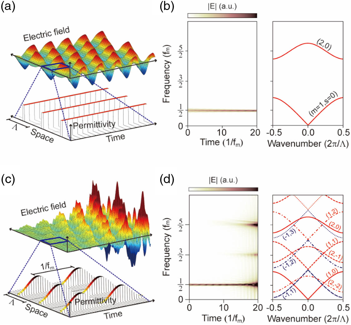
    Fig. 1. Spatiotemporal field evolution of the lowest-order PC mode. (a) Permittivity profile in space-time for a time-invariant PC, and spatiotemporal electric field distribution of a lowest order PC eigenmode. (b) Time-resolved spectral amplitude (left panel) and dispersion diagram (right panel) of the time-invariant PC. The spectral amplitude is invariant with respect to time (left panel). Note that the frequency axis is normalized to the modulation frequency. (c) Permittivity profile in space-time for an SC and spatiotemporal electric field distribution of the lowest-order PC eigenmode. The originally launched PC eigenmode has evolved into a mode with growing intensity. (d) Time-resolved spectral amplitude (left panel) and PC dispersion curve along with its temporally scattered bands (right panel). Three major frequency components are seen clearly in the left panel. The line color and style represent the sign of the frequency and mixing order, respectively.
    Dispersion diagrams of a PC and SCs. (a) Permittivity profile in space-time (top panel) and dispersion diagram of the PC. The two lowest bands are clearly shown in the middle and bottom panels. (b) Permittivity profile in space-time and dispersion diagram of the SC modulated at fm=f0. Red lines are the dispersion curves calculated using the ST-PWEM. The lowest panels are the imaginary parts of the eigenfrequencies corresponding to the MBGs denoted by A and B in the middle panel. The MBGs denoted by A and B are classified as (1, 0; −1, 1) and (1, 1; −1, 2), respectively. (c) Permittivity profile in space-time and dispersion diagram of the SC modulated at fm=3f0/2. The MBGs denoted by A and B are classified as (1, 0; −2, 2) and (1, 0; −1, 1), respectively. (d) Permittivity profile in space-time and dispersion diagram of the SC modulated at fm=5f0/2. The MBG denoted by A is classified as (1, 0; −3, 2). For comparison, one of the EBGs is shown and denoted by B. (e) Permittivity profile in space-time and dispersion diagram of the SC modulated at fm=3f0. The MBGs denoted by A and B are classified as (1, 0; −2, 1) and (1, 0; −3, 2), respectively.
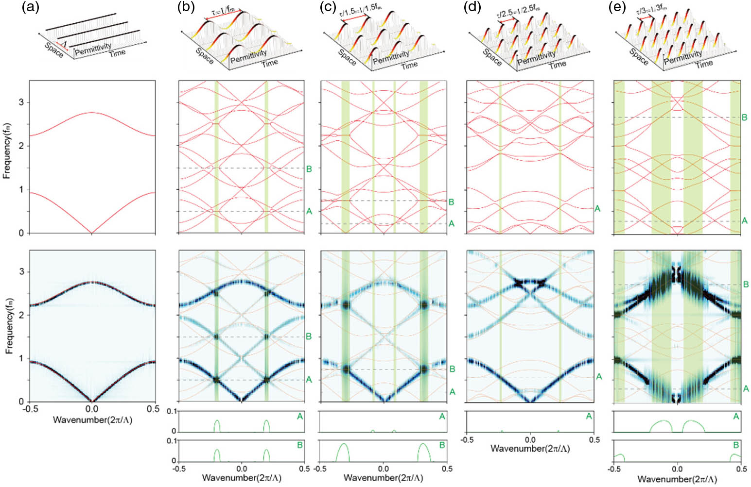
    Fig. 2. Dispersion diagrams of a PC and SCs. (a) Permittivity profile in space-time (top panel) and dispersion diagram of the PC. The two lowest bands are clearly shown in the middle and bottom panels. (b) Permittivity profile in space-time and dispersion diagram of the SC modulated at fm=f0. Red lines are the dispersion curves calculated using the ST-PWEM. The lowest panels are the imaginary parts of the eigenfrequencies corresponding to the MBGs denoted by A and B in the middle panel. The MBGs denoted by A and B are classified as (1, 0; 1, 1) and (1, 1; 1, 2), respectively. (c) Permittivity profile in space-time and dispersion diagram of the SC modulated at fm=3f0/2. The MBGs denoted by A and B are classified as (1, 0; 2, 2) and (1, 0; 1, 1), respectively. (d) Permittivity profile in space-time and dispersion diagram of the SC modulated at fm=5f0/2. The MBG denoted by A is classified as (1, 0; 3, 2). For comparison, one of the EBGs is shown and denoted by B. (e) Permittivity profile in space-time and dispersion diagram of the SC modulated at fm=3f0. The MBGs denoted by A and B are classified as (1, 0; 2, 1) and (1, 0; 3, 2), respectively.
    Spatiotemporal mode field profiles at the edges of an MBG. (a) Dispersion diagram of the SC modulated at fm=f0. (b) Spatiotemporal permittivity profile of the PC unit cell used to calculate the dispersion curves. The parameters are identical to those used to calculate the dispersion curves in Fig. 2(b). (c) Numerically calculated spatiotemporal mode field profile at the lower wavenumber edge of the MBG. (d) Numerically calculated spatiotemporal mode field profile at the higher wavenumber edge of the MBG.
    Fig. 3. Spatiotemporal mode field profiles at the edges of an MBG. (a) Dispersion diagram of the SC modulated at fm=f0. (b) Spatiotemporal permittivity profile of the PC unit cell used to calculate the dispersion curves. The parameters are identical to those used to calculate the dispersion curves in Fig. 2(b). (c) Numerically calculated spatiotemporal mode field profile at the lower wavenumber edge of the MBG. (d) Numerically calculated spatiotemporal mode field profile at the higher wavenumber edge of the MBG.
    Emergence of parametric oscillations at the MBG. (a) Schematic of a finite-sized SC (left panel). The electric fields of incident and transmitted waves are represented by Ei→ and Et→, respectively. The permittivities of constituting slabs are sinusoidally modulated in phase (right panel). (b) Transmitted field amplitude spectra for N=8 plotted as a function of the normalized permittivity variation. Two oscillating spectra are scaled to fit in the plot. (c) Transmitted field amplitude spectra for N=10 plotted as a function of the normalized permittivity variation. Four oscillating spectra are scaled to fit in the plot. The frequency of the input wave is set to 1.5 GHz for both (b) and (c). (d) Temporal field growth rates as a function of the normalized permittivity variation and the number of unit cells in the finite-sized SC. The temporal field growth rates are plotted for frequencies corresponding to three MBGs at fm/2, 3fm/2, and 5fm/2.
    Fig. 4. Emergence of parametric oscillations at the MBG. (a) Schematic of a finite-sized SC (left panel). The electric fields of incident and transmitted waves are represented by Ei and Et, respectively. The permittivities of constituting slabs are sinusoidally modulated in phase (right panel). (b) Transmitted field amplitude spectra for N=8 plotted as a function of the normalized permittivity variation. Two oscillating spectra are scaled to fit in the plot. (c) Transmitted field amplitude spectra for N=10 plotted as a function of the normalized permittivity variation. Four oscillating spectra are scaled to fit in the plot. The frequency of the input wave is set to 1.5 GHz for both (b) and (c). (d) Temporal field growth rates as a function of the normalized permittivity variation and the number of unit cells in the finite-sized SC. The temporal field growth rates are plotted for frequencies corresponding to three MBGs at fm/2, 3fm/2, and 5fm/2.
    Temporal evolution of frequency mixing and parametric oscillation. (a) Temporal evolution of the total transmitted field above the transition threshold. Two characteristic parameters, ttp and g1, describe the temporal evolution of the total transmitted field. (b) Time-resolved spectral amplitude of the total transmitted field above the transition threshold. For this particular detuned input case (Δf=f0−fm/2=0.5 GHz), the temporal evolution of the total transmitted field is initially dominated by frequency mixing but eventually governed by parametric oscillations. The tipping point time ttp is nonzero for this case. (c) Tipping point time ttp, plotted as a function of the input frequency. In this example, the first MBG frequency is 1.0 GHz. When the input frequency is tuned exactly to the first MBG frequency, the tipping point time becomes zero. (d) The temporal field growth rate g1 is shown to be independent of the input frequency.
    Fig. 5. Temporal evolution of frequency mixing and parametric oscillation. (a) Temporal evolution of the total transmitted field above the transition threshold. Two characteristic parameters, ttp and g1, describe the temporal evolution of the total transmitted field. (b) Time-resolved spectral amplitude of the total transmitted field above the transition threshold. For this particular detuned input case (Δf=f0fm/2=0.5  GHz), the temporal evolution of the total transmitted field is initially dominated by frequency mixing but eventually governed by parametric oscillations. The tipping point time ttp is nonzero for this case. (c) Tipping point time ttp, plotted as a function of the input frequency. In this example, the first MBG frequency is 1.0 GHz. When the input frequency is tuned exactly to the first MBG frequency, the tipping point time becomes zero. (d) The temporal field growth rate g1 is shown to be independent of the input frequency.
    Asymmetric formation of MBGs and direction-dependent radiation of oscillations. (a) Permittivity profile in space-time (top panel) and dispersion diagrams (middle and bottom panels) of the SC modulated at fm=f0 and K=−2π/8Λ. Red lines in the middle panel are calculated using the ST-PWEM. The mixing order is limited up to ±2. The MBGs denoted by A and B can be labeled with (1, 0; −1, 1; +) and (1, 0; −1, 1; −), respectively. The two-dimensional Fourier-transformed field is plotted in the bottom panel. The scattering by the traveling-wave-type modulation is represented by the yellow arrow. (b) Permittivity profile in space-time (top panel) and dispersion diagrams (middle and bottom panels) of the SC with K=2π/8Λ. (c) Permittivity profile in space-time (top panel) and dispersion diagrams (middle and bottom panels) of the SC with K=−2π/4Λ. (d) Permittivity profile in space-time (top panel) and dispersion diagrams (middle and bottom panels) of the SC with K=2π/4Λ. (e) Temporal evolution of the field radiated from the input and output facets of the finite-sized SC (N=56). (f) Amplitude spectra of the forward and backward radiating fields from the finite-sized SC.
    Fig. 6. Asymmetric formation of MBGs and direction-dependent radiation of oscillations. (a) Permittivity profile in space-time (top panel) and dispersion diagrams (middle and bottom panels) of the SC modulated at fm=f0 and K=2π/8Λ. Red lines in the middle panel are calculated using the ST-PWEM. The mixing order is limited up to ±2. The MBGs denoted by A and B can be labeled with (1, 0; 1, 1; +) and (1, 0; 1, 1; −), respectively. The two-dimensional Fourier-transformed field is plotted in the bottom panel. The scattering by the traveling-wave-type modulation is represented by the yellow arrow. (b) Permittivity profile in space-time (top panel) and dispersion diagrams (middle and bottom panels) of the SC with K=2π/8Λ. (c) Permittivity profile in space-time (top panel) and dispersion diagrams (middle and bottom panels) of the SC with K=2π/4Λ. (d) Permittivity profile in space-time (top panel) and dispersion diagrams (middle and bottom panels) of the SC with K=2π/4Λ. (e) Temporal evolution of the field radiated from the input and output facets of the finite-sized SC (N=56). (f) Amplitude spectra of the forward and backward radiating fields from the finite-sized SC.
    Seojoo Lee, Jagang Park, Hyukjoon Cho, Yifan Wang, Brian Kim, Chiara Daraio, Bumki Min. Parametric oscillation of electromagnetic waves in momentum band gaps of a spatiotemporal crystal[J]. Photonics Research, 2021, 9(2): 142
    Download Citation