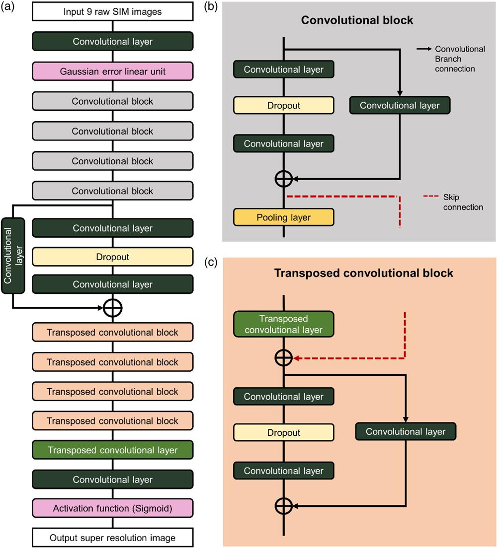
Fig. 1. Network architecture of VDL-SIM. (a) The architecture of VDL-SIM. It contains four CBs and four transposed CBs. (b) The composition of a CB. It consists of two convolutional layers and a dropout layer connected to a convolution branch and then pooled. (c) The composition of a transposed CB. It consists of a transposed convolutional layer, a skip connection, and a CB without pooling operation.

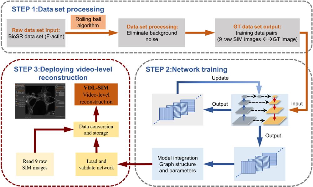
Fig. 2. VDL-SIM video-level reconstruction method pipeline. (STEP1) Data set processing. The training data pairs are obtained after performing the background removal on the raw data set with the rolling ball algorithm. The effect of the rolling ball algorithm on VDL-SIM is given in Sec. S3 of the Supplementary Material. (STEP2) Network training process. The data are fed to the network for training, updating the weights until convergence. Afterward, model integration is performed to generate files containing graph definitions and weight parameters. (STEP3) Software side deployment of SIM video-level reconstruction. The model is loaded for validation followed by reading in the fast-captured images to reconstruct.

Fig. 3. Comparison of performance for deep-learning SIM SR reconstruction. (a) Comparison table of reconstruction speeds for three FOVs, with a camera pixel size of 65 nm. (b) A more visual histogram presentation of the reconstruction speeds in (a). (c) Comparison of the quality of three metrics of reconstructed images. (d) Data for three metrics: MSE, PNSR, and SSIM.

Fig. 4. Video-level SIM reconstruction result presentation of VDL-SIM. (a) Video-level reconstructed microtubule results at 1, 24, and 47 s under different lateral positions. (b) Video-level reconstructed F-actin results at 10, 11, and 12 s under different axial positions. The exposure time of (a) and (b) are set to 15 ms, and the FOV is 512pixel×512pixel. (c) VDL-SIM reconstruction software interface. Scale bars, 5 µm.

Fig. 5. Comparison of VDL-SIM algorithm with DFCAN and ML-SIM algorithms for imaging F-actin structures under three SNR conditions. (a) Reconstruction images and evaluation metrics comparison of three deep-learning algorithms under an excitation wavelength of 640 nm and SNR of 24.04 imaging conditions. (b) and (c) with SNRs of 21.29 and 16.72, respectively; the rest of the imaging conditions are the same as that in (a). The GT images referenced for the metrics calculation are provided by the HiFi algorithm with sufficient laser dose. Scale bars, 2 µm (larger image) and 1 µm (boxed magnified image).

Fig. 6. Comparison of SIM SR reconstruction of mitochondrial structures at low SNR levels. (a) Imaging comparison of VDL-SIM with deep-learning DFCAN and ML-SIM algorithms under conditions with SNR of 21.83. The excitation wavelength is 488 nm. (b) The WF image and the conventional SIM algorithm HiFi and IM imaging results are shown under the same imaging conditions as that in (a). (c) Comparison of VDL-SIM, DFCAN, and ML-SIM normalized intensity profiles of the central hollow in the boxed magnified images. (d) Comparison of VDL-SIM, HiFi, and IM normalized intensity profiles of the central hollow in the box magnified images. (e) and (f) Comparison of the effect of VDL-SIM, HiFi, and IM algorithms to reconstruct mitochondria at SNRs of 17.92 and 13.92, respectively. Scale bars, 2 µm (large images) and 1 µm (boxed magnified images).

Fig. 7. VDL-SIM imaging of living specimens. (a) VDL-SIM reconstructed images of dynamic ER for 0–1.62 s. (b) VDL-SIM reconstructed images of dynamic microtubules for 0–1.62 s. Scale bars are 1 µm. The excitation wavelength of microtubules is 488 nm; ER is 561 nm.