Structural illumination microscopy (SIM) is an optical super-resolution (SR) imaging technique that uses specific illumination patterns to excite fluorescent samples, producing interference patterns that contain detailed information about the structure of the sample. Such detailed information is not observable in conventional diffraction-limited imaging. The basic principle of SIM is that the superimposed sample spectra are generated using sinusoidal illumination patterns, which can be reconstructed as SR images by separating and relocating the superimposed spectra to the correct frequency space^[1]. Taking one-directional SR reconstruction as an example, the superimposed spectra are shifted to three positions +k0,0,−k0 in the frequency domain. In order to separate the three spectra, three linear equations based on three phase-shifted images are built. To achieve two-dimensional (2D) resolution improvement, the pattern direction needs to be rotated 3 times to collect nine raw images^[2]. This is then followed by the Fourier transform of the reconstructed spectrum back to the spatial domain, resulting in images with doubled resolution^[3,4]. The introduction of this technique brings a breakthrough in optical microscopy, transcending the conventional diffraction limitations and providing higher-resolution view of sample structure.

However, with the traditional SIM reconstruction algorithm, it is difficult to accurately estimate the illumination parameters under suboptimal imaging conditions, resulting in reconstructed images plagued by artifacts. The above limitations are especially prominent in low signal-to-noise ratio (SNR) imaging conditions in which the sample structure is prone to be reconstructed erroneously as noise may introduce obvious artifacts. In such cases, neural networks have excellent ability to infer complex features; with the help of deep-learning methods, a neural network can learn complex structural features of images autonomously, thereby addressing the SIM problem of poor robustness on imaging noise^[5–7]. However, the numerous parameter calculations make the single reconstruction time of existing deep-learning SIM methods in the typical order of seconds^[8], limiting their application in living SR observation of rapid movements. Capturing structural changes of living cells in a real-time manner and with high quality is crucial for our understanding of biological processes, and for discovering and analyzing pathologies. In the past few years, researchers have introduced various techniques to improve the real-time imaging capability of microscopy techniques, such as real-time non-deep-learning SIM reconstruction based on GPU enhancement^[2], accelerated non-deep-learning SIM reconstruction techniques based on simplified workflow^[9,10], and fast image denoising based on neural networks^[11,12].

Inspired by these work, here we propose a deep-learning-based method for video-level and real-time high-fidelity SR SIM reconstruction, termed video-level deep-learning SIM (VDL-SIM), which integrates lightweight neural network construction and software deployment into a single unified process to achieve the goal of video-level low SNR reconstruction and to address the problems of slow speed and poor noise robustness. VDL-SIM employs an end-to-end residual^[13] U-Net^[14–16] lightweight network via a multilevel nonlinear transformation to capture the nonlinear relationship between signal and noise from massive data, which is difficult to capture by traditional SIM algorithms. The advantages of VDL-SIM are also reflected in the reconstruction speed. Through a subtle structural design, VDL-SIM possesses both the multiscale effective information capturing capability of U-Net and the deep understanding and training capability of residual networks. Based on the synergy of the two architectures, we cut down the number of network channels and trade off the performance of the VDL-SIM model to accelerate the imaging while maintaining high-fidelity output. Joined with the hardware system timing^[17], VDL-SIM can reach 47 frame/s, corresponding to 15- to 33-fold improvement compared to existing deep-learning SIM reconstruction algorithms. VDL-SIM is thus helpful for observing live samples with higher resolution, lower photobleaching, and lower phototoxicity, providing a powerful tool for SR biological studies.

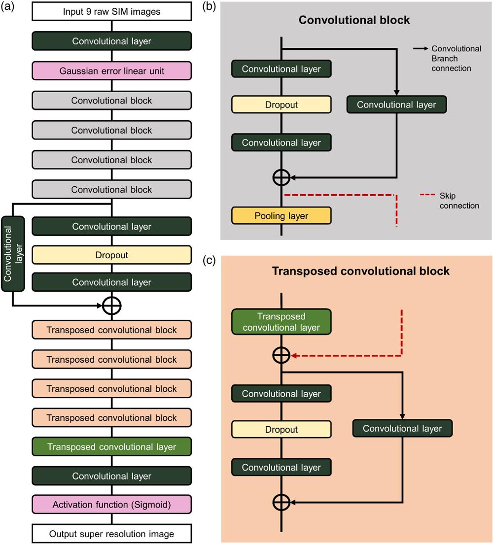
The network architecture of VDL-SIM is shown in Fig. 1(a), which begins with a convolutional layer and a Gaussian error linear unit^[18]. The output of the Gaussian error linear unit is followed by four identical convolutional blocks (CBs). The structure of the CB is shown in Fig. 1(b); each CB consists of two convolutional layers and a dropout layer connected to a convolutional branch followed by a pooling operation^[19]. The operation of the CB is given as CB(x)=Pooling(y).(1)

The intermediate variable y is defined as y=Conv{x}+Conv{Drop(Conv{x})},(2)where x denotes the input feature maps of the CB, Pooling represents the pooling layer operation, Conv represents the convolutional layer operation, and Drop represents the dropout layer operation.

The output of the last CB is sent to the convolutional layers and the dropout layer and then connected to its own convolutional skip. Following the output are four identical transposed convolutional blocks (TCBs), as shown in Fig. 1(c). The TCB operation is denoted as TCB(x)=Conv{ConvT{x}+y}+Conv{Drop(Conv{ConvT{x}+y})},(3)where x denotes the input feature maps of the TCB, ConvT represents the transposed convolutional layer operation, and y is defined in Eq. (2) above.

The final TCB output then passes through a transposed convolutional layer before the image is upgraded to the same size as the ground truth (GT) image using the convolution and sigmoid activation function to accommodate the inferred high-frequency information. Finally, the network outputs a monochrome gray-scale SR image.

Our VDL-SIM network based on lightweight residual U-Net is more computationally efficient compared to other networks, such as the generative adversarial network (GAN). Generators and discriminators in GAN need to compete and co-train with each other, which makes the training process more complex and slower to converge^[20]. In contrast, U-Net is known for its multiscale features and efficient upsampling^[14–16], and the residual network improves the understanding of image structure through depth and jump-connection mechanisms^[13]. The combination of both thus allows the VDL-SIM network to be easier to train and converge quickly while maintaining high-quality outputs. We further simplify the VDL-SIM model by pruning the number of network channels and present the selection process for pruning channels in Sec. S1 of Supplementary Material to balance imaging speed and quality. The channel pruning could reduce the number of weight parameters in the model, thereby significantly reducing storage and computational costs. In addition, pruning the number of channels also helps to remove redundant and unnecessary information that might be learned during training, making the VDL-SIM model more compact and robust. As a result, the lightweight VDL-SIM network could produce high-quality results with high time-efficiency without the need for complex adversarial training.

The VDL-SIM network is trained with the Adam optimizer^[21], allowing iterative updating of the neural network weights based on the training data, with the advantage of efficient computability. The objective function of the network is defined as a combination of mean square error (MSE) and structural similarity index measure (SSIM) losses^[20]. The MSE loss ensures pixel accuracy, and the SSIM loss enhances the structural similarity of the output. In each training iteration, the initial learning rate is set to 0.0001. The network then learns at a 50% decay rate, and the training is terminated until the learning rate reaches the minimum value of 0.00001. Twenty thousand epochs are trained, and the batch size for each round of training is 2. The network is trained using NVIDIA GeForce RTX 3050Ti GPUs. It is important to note that the storage and processing space occupied by a training set with too large of an image size may exceed the memory capacity of the device, affecting the forward or backward propagation of the network. In our work, the input image size for training is 128pixel×128pixel, with a pixel size of 65 nm. Taking the F-actin data set as an example, 20,000 iterations took about 1 h.

The reconstruction pipeline of VDL-SIM is shown in Fig. 2, which integrates the three steps of data set processing, network training, and deploying video-level reconstruction into a unified process. The network is utilized with C++ hardware acceleration features^[17] to enhance the speed of SR reconstruction and provide a software interface.

We choose the more complex structure of F-actin in the open-source BioSR data set^[16] as the training data source due to its high generalizability. The choice of the structure for training the data set is discussed in detail in Sec. S2 of the Supplementary Material. Note that in order to improve the reconstruction, we utilize the rolling ball algorithm^[22] to act on the GT images in the training data set, pairing the background-removed GT images with their corresponding nine raw SIM images, forming data pairs. We provide the principle of the rolling ball algorithm, and our selection process, in Sec. S3 of the Supplementary Material. After background suppression processing, the information in the image is more focused, which allows the network to better understand the structural features while reducing the computational resource requirements. STEP1 in Fig. 2 shows the process of training data set acquisition. More details of the processing are given in Sec. S2 of the Supplementary Material. STEP2 is the network training (Fig. 2, STEP2). The nine raw SIM images are provided as input, and the output is compared with the GT images to update the network weights by calculating the joint loss of pixel accuracy and structural similarity. After training convergence, the optimal graph structure and weight parameters of the network are saved and integrated with the model to be deployable. In the final reconstruction step, we load and validate the integrated network, feed a series of nine raw SIM images into the storage matrix, and utilize GPU to accelerate the network computation to achieve video-level microscopic reconstruction (Fig. 2, STEP3).

The basic software functions include camera timing control, laser control, sample stage control, and reconstruction control^[23–25]. Users can perform DVL-SIM reconstruction by selecting the excitation light wavelength, entering the exposure time and laser intensity, pressing the deep learning video-level reconstruction button, and selecting the appropriate observation area by controlling the motorized displacement table knob. The experimental data were mainly acquired using a home-made high-speed SIM system^[17,26] based on electro-optic modulators (EOMs) and a scanning galvanometer system, with a multicolor laser serving as the light source. EOMs (Thorlabs, EO-PM-NR-C4) and scanning galvanometer systems (Cambridge Technology, 8310 K) are used to generate and change the structured illumination pattern. The modulated sample information is recorded as a single-phase image through an objective lens (Nikon, 100×/NA 1.49) and a digital sCMOS camera (Hamamatsu, ORCA-Flash4.0 V3). The raw images obtained have a pixel size of 65 nm.

Speed comparison of video-level SIM reconstruction by VDL-SIM and existing SIM deep-learning algorithms is shown in Figs. 3(a) and 3(b). The field-of-view (FOV) selection supports 128pixel×128pixel to 512pixel×512pixel, which can be adjusted according to user requirements. Three algorithms of VDL-SIM, DFCAN^[20], and ML-SIM^[13] are used for the comparison. The test graphics card is NVIDIA GeForce RTX 3050Ti GPU and the camera used is Hamamatsu, ORCA-Flash4.0 V3, with a pixel size of 65 nm. As shown in Fig. 3(a), the VDL-SIM network improves the speed ranging from 6- to 15-fold over the ML-SIM algorithms. Specifically, compared to the DFCAN network, the difference becomes even more pronounced under 128pixel×128pixel, where the speed improvement reaches 33-fold. Our work accelerates deep-learning SIM SR reconstruction and achieves video-level goals.

Along with improving the reconstruction speed, we analyze the imaging quality of different deep-learning algorithms. Taking the reconstructed image of a HiFi algorithm^[27] under sufficient laser dose as the GT image, we compared the three reconstruction metrics: peak signal-to-noise ratio (PNSR), structural similarity index (SSIM), and mean squared error (MSE) of DFCAN, ML-SIM, and VDL-SIM algorithms at different SNRs. As shown in Fig. 3(d), the image fidelity of ML-SIM reconstruction under the same level of SNR is weak, evinced by its excessive MSE value, and both PSNR and SSIM index values are the minimum; especially at the very low SNR of 4.87, the structural similarity is less than 0.1. On the other hand, VDL-SIM has the advantage in the three indices; as shown in Fig. 3(c), the PSNR and SSIM can be maintained at a better level; also, the MSE is the smallest. VDL-SIM still maintains the reconstruction effect of about 50%, even at the 4.87 SNR level. Our analysis illustrates that VDL-SIM can still be robustly reconstructed at deficient light doses, which provides a new possibility for lower phototoxicity SIM imaging. We will present the reconstructed images later in Sec. 3.3. Although VDL-SIM has better reconstruction ability at lower SNR, we admit that VDL-SIM’s reconstruction ability at high SNR is not eminently outstanding, and we can expect further improvement of VDL-SIM’s performance in future work.

We then use microtubules and F-actin structures to demonstrate the video-level reconstruction and display capabilities of VDL-SIM. The excitation light wavelengths of the microtubules and F-actin are 561 and 640 nm, respectively. Figure 4(a) shows the video-level reconstructed images of the microtubule samples under successive lateral positions at the same focus. By contrast, Fig. 4(b) shows the video-level reconstructed images of the F-actin samples under successive axial positions at the same lateral position. As we can see, VDL-SIM can maintain high-fidelity reconstruction at the focus position as we move the sample position or the focal plane. For better visualization, we present an example of video-level reconstruction of microtubule structures by VDL-SIM in Video 1. Figure 4(c) shows the running VDL-SIM reconstruction software interface. The right panel supports offline reconstruction. The left panel supports the parameter setting, including excitation light wavelengths, camera exposure time, and FOV sizes. The middle panel shows the SR video stream for SIM video-level reconstruction.

In the above two experiments, the exposure time per raw image is set to 15 ms, and the camera used is Hamamatsu, ORCA-Flash4.0 V3, which can capture images at the maximum speed of 400 frame/s. Since video-level SIM imaging requires fast image acquisition, reconstruction, and display simultaneously, if the exposure time is not set properly, it will lead to the presence of residual images from the previous region. Therefore, when utilizing VDL-SIM for video-level reconstruction, it is important to match the exposure time and reconstruction speed to avoid the problem of display delay and jamming. Taking the 512×512 FOV as an example, the exposure time needs to be set below 15–20 ms.

In practical biological applications, which often involve fast imaging, it is common practice to set the laser intensity and exposure time at lower levels. This is done to mitigate potential issues related to photobleaching and phototoxicity, resulting in captured images with a low SNR. Traditional SIM algorithms have a high-fidelity SR imaging capability at high SNR conditions, but are prone to introduce artifacts and even fail to reconstruct at low SNR due to inaccurate parameter estimation. Benefiting from the robust learning ability of the network model, VDL-SIM could address the issue and achieve high-quality video-level reconstruction under low SNR.

To demonstrate the robust reconstruction ability of VDL-SIM, we compare the reconstructed images and evaluation indices of F-actin structure among VDL-SIM, DFCAN, and ML-SIM at three SNR levels. In Fig. 5(a) with SNR equal to 24.04, the structural similarity index of VDL-SIM reaches 78%; however, DFCAN and ML-SIM are only around 50%, while VDL-SIM maintains a higher PSNR and the lowest MSE of the three algorithms. With the decrease of SNR, the ML-SIM image is no longer able to perform effective SR reconstruction, with more artifacts, and DFCAN is also unable to distinguish two close microtubules, whereas VDL-SIM can do the job [Figs. 5(b) and 5(c)]. In particular, at SNR equal to 16.72, the MSE value of ML-SIM is about 10 times that of VDL-SIM, while DFCAN’s SSIM is only half of that.

We demonstrate the advantages of VDL-SIM over the deep-learning SIM algorithms DFCAN and ML-SIM, both in terms of reconstruction speed (as described in Sec. 3.1) and robust reconstruction capability. This advantage is also valid for mitochondrial structures. Figure 6(a) demonstrates the imaging results of DFCAN, ML-SIM, and VDL-SIM under the SNR of the 21.83 conditions. It can be seen that in the magnified image, ML-SIM has more severe ringing artifacts, and VDL-SIM distinguishes the middle hollow much more clearly than DFCAN, which is evident as shown in the lower central value of the normalized intensity of VDL-SIM in Fig. 6(c). More notably, the advantage of VDL-SIM’s high-fidelity robust reconstruction ability at low SNR will be even more prominent when compared with traditional SIM algorithms, as we further illustrate by comparing VDL-SIM with the traditional SIM algorithms inverse matrix-SIM^[28] (IM) and high-fidelity SIM^[27] (HiFi).

At low laser intensities, the mitochondria under SNR of 21.83, 17.92, and 13.92 conditions were imaged by the conventional SIM algorithms HiFi and IM, respectively. As shown in Figs. 6(b), 6(e), and 6(f), IM at low SNR tends to reconstruct the scattered dots, and it is also difficult for HiFi to recognize the mitochondrial structure, as their normalized intensity shows an irregular trend in Fig. 6(d). This is caused by the inability of the conventional algorithm to perform correct parameter estimation under poorer imaging conditions. However, our VDL-SIM algorithm still recovers the sample details better at the same SNR level. Additionally, we demonstrate the ability of VDL-SIM to reconstruct biological structures under extremely low SNR imaging conditions (SNR<10), in Sec. S4 of the Supplementary Material. In application scenarios of living specimen imaging, where low SNR imaging conditions are essential for the goal of maintaining the physiological state, VDL-SIM can serve as a complementary technique for such application scenarios to give the observer a reference of the biological structure.

To further visualize the effect of video-level VDL-SIM reconstruction, we provide a comparison video for wide-field (WF), HiFi, and VDL-SIM reconstruction under low SNR conditions. Quantitative analysis for the imaging performance of the video frames was also done. See Video 2 and Fig. S5 of the Supplementary Material. The VDL-SIM algorithm enables robust reconstruction at low SNR, provides a new technique that can be applied under challenging imaging conditions, fulfills the blank of traditional SIM algorithms in this application area, and offers the possibility of further reducing the phototoxicity of SIM imaging.

Next, we demonstrate the VDL-SIM’s living specimen imaging task. The endoplasmic reticulum (ER) is responsible for the transportation of substances in and out of the cell, linking the nucleus with the cytoplasm, which is a major cellular structure. Microtubules are essential for maintaining cellular morphology and participating in the transportation of cellular materials. Some existing SR imaging techniques require SR reconstruction by high light intensity and long exposure time, which are prone to phototoxicity in living cells. In this work, we applied the video-level imaging technique of VDL-SIM to characterize the dynamics of microtubules and ER, with the exposure time of 20 ms for a single image.

As shown in Fig. 7, the ER membrane stretches and coalesces over time during a sustained imaging time of 1.62 s. Similarly, two parallel microtubules are clearly observed to be stretched apart by VDL-SIM. VDL-SIM is capable of capturing even fleeting and subtle biological processes, confirming the usability of VDL-SIM in practical experiments.

We demonstrate and validate VDL-SIM, a video-level high-fidelity SIM SR reconstruction method based on a deep-learning neural network. The method designs a clever network structure that synergizes two architectures, U-Net and residual network, which enables VDL-SIM to have better information capturing and deep understanding training capabilities. Meanwhile, under the principle of a trade-off between reconstruction performance and speed, our work utilizes the method of pruning the number of network channels to speed up the imaging speed. To improve the VDL-SIM reconstruction effect under challenging imaging conditions, we utilize the rolling ball algorithm to preprocess the data set in advance. Interweaving network construction and software deployment^[29] into a unified process, we finally achieve video-level high-fidelity deep-learning SIM reconstruction with 47 frame/s (256×256 FOV). The high-fidelity advantage of VDL-SIM reconstruction is obvious. We compare the reconstructed images from DFCAN and ML-SIM in deep-learning algorithms with that of VDL-SIM. Our work achieves faster reconstruction speed and better quality reconstruction indices. The advantage is even more significant at low SNR experimental conditions, when traditional HiFi and IM algorithms have difficulty in correctly performing parameter estimation, but VDL-SIM is still able to achieve robust SR reconstruction. Our proposed VDL-SIM algorithm can overcome the tough photobleaching and phototoxicity imaging conditions, filling the blank of traditional SIM algorithms in low SNR applications, and providing a powerful tool to further reduce the phototoxicity of SIM imaging for application to the observation of living samples and SR biological research. However, it must be admitted that there is still potential to improve the resolution of VDL-SIM, which is not outstanding at high SNR and suffers from missing information at extremely low SNRs. As well, how to solve the credibility problem of deep learning in applications will be a persistent problem. These issues may subsequently be further relieved by combining mathematical prior knowledge, such as sparse constraints^[30,31] and physical imaging models^[10,32,33].

References

[5] E. Moen et al. Deep learning for cellular image analysis. Nat. Methods, 16, 1233(2019).
[18] D. Hendrycks, K. Gimpel. Gaussian error linear units (GELUs)(2023).
[21] D. P. Kingma, J. Ba. Adam: a method for stochastic optimization(2017).
[22] S. R. Sternberg. Biomedical image processing. Computer, 16, 22(1983).
[34] https://github.com/WenjieLab/Deep-learning-based-real-time-SIM
Set citation alerts for the article
Please enter your email address
© Copyright 2018-2021 | Chinese Laser Press. All Rights Reserved 沪ICP备15018463号-20