Jinhua Li, Xiangdong Zhang, "Electric field tunable strong transverse light current from nanoparticles embedded in liquid crystal," Photonics Res. 6, 630 (2018)
Copy Citation Text
We present an exact solution to the problem of electromagnetic scattering by nanosphere clusters embedded in a liquid crystal cell, based on the Mie theory. The dependence of the scattering property on the structure parameters is investigated in detail. It is shown that strong transverse light currents at the optical frequency can be obtained from these complex structures. Furthermore, we find that sign reversal of the transverse light current can be realized by changing frequency and voltage. The physical origins of these phenomena have been analyzed. The transverse light current for subwavelength nanoscale dimensions is of practical significance. Thus, the application of these phenomena to optical devices is anticipated.
In recent years there has been a great deal of interest in studying the photonic Hall effect, which is a manifestation of a magnetically induced transverse current in light transport analogous to the classical Hall effect in the transport of electrons [1]. Such an effect was theoretically predicted about 20 years ago by van Tiggelen [1], and experimentally confirmed by Rikken and van Tiggelen [2]. The photonic Hall effect finds its origin in the magnetically induced changes of the optical parameters [3–5]. The theoretical research takes into account the anisotropy of the optical parameters using point-like scatters [6,7]. Based on perturbation theory, Lacoste et al.[8] have addressed the issue of whether or not there is a photonic Hall effect for one single Mie scatterer. Subsequently, the exact Mie-type solutions to such a problem have been presented, and a photonic Hall effect from the Mie scatterers has been demonstrated [9]. However, these investigations have focused on magnetized materials or nonmagnetic media in the presence of the external magnetic field. Accordingly, the phenomenon is difficult to observe at visible and near-infrared frequencies because the magnetic susceptibility of all natural materials tails off at microwave frequencies. Recently, sign inversion of the effective Hall coefficient in chainmail-like metamaterials has also been predicted theoretically [10] and observed experimentally in the infrared frequency region [11]. In fact, the metamaterials in the visible frequency region are also very difficult to prepare.
On the other hand, the occurrence of an electric-field-driven transverse photon current in light scattering by a single metallic sphere coated with a liquid crystal (LC) shell was recently reported [12]. The advantage of such a method is that the phenomenon can not only be observed at the optical frequencies but also is tunable by the voltage instead of magnetic fields. However, the transverse optical signals generated in this way are very weak, and the modulation range by the electric field is also very small. The problem is whether electric-field-tunable strong transverse light current can be observed at the optical frequency and how.
Motivated by these investigations, in this work we consider the problem of electromagnetic scattering by nanosphere clusters embedded in LC shells. Such a scattering problem can be discussed in principle using the recognized numerical boundary element method, finite difference time domain, or finite element method software. However, it is very difficult to obtain convergence using these methods when the distances between the nanospheres are smaller than 1 to 2 nm.
Sign up for Photonics Research TOC. Get the latest issue of Photonics Research delivered right to you!Sign up now
A multiple scattering method based on Mie theory is best suited for a finite collection of spheres or cylinders with a continuous incident wave of fixed frequency [13–17]. For spheres or cylinders, the scattering property of the individual scatter can be obtained analytically, relating the scattered fields to the incident fields. The total field, which includes the incident plus the multiple scattered fields, can then be obtained by solving a linear system of equations whose size is proportional to the number of scatters in the system. Both near- and far-field patterns can be obtained straightforwardly. Thus, such a method is a very efficient way of handling the scattering problem of a finite sample containing spheres or cylinders; it is capable of reproducing accurately the experimental transmission data, which should be regarded as an exact numerical simulation. However, the existing theories are only for cases of nanoparticle clusters embedded in the isotropic background. As for the problem of electromagnetic scattering by nanoparticle clusters embedded in the anisotropic background, no theory has been provided so far.
In this work, we use Mie theory to study and solve the problem of electromagnetic scattering by nanosphere clusters embedded in LC cells. Our calculations show that strong transverse light currents in the optical frequency can be obtained from these complex structures, and sign reversal of the transverse light current can be realized by changing frequency and voltage. The rest of this paper is arranged as follows. In Section 2, we provide a multiple scattering theory for nanosphere clusters embedded in LC cells. The results and discussion are shown in Section 3, and a summary is given in Section 4.
2. MULTIPLE SCATTERING THEORY FOR NANOSPHERE CLUSTERS EMBEDDED IN LC CELLS
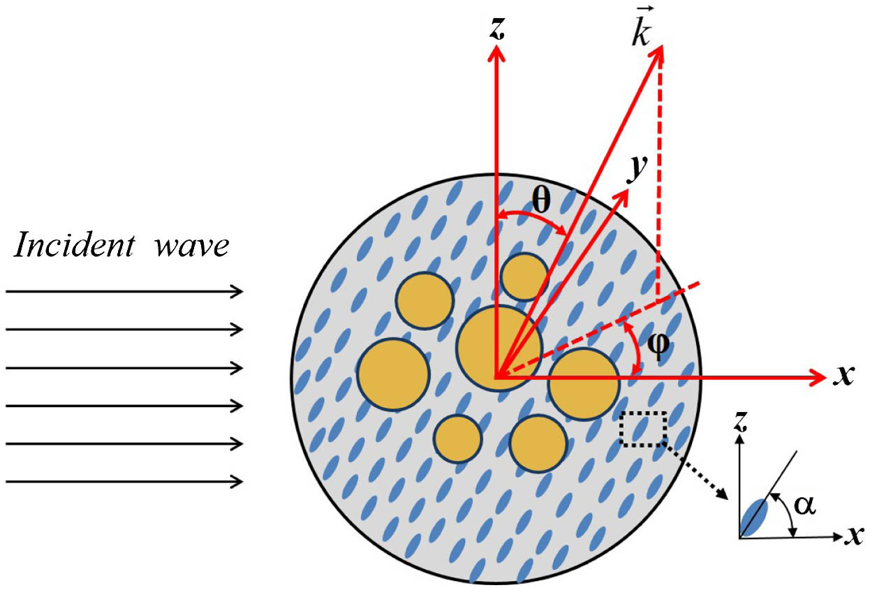
We consider an ensemble of spheres embedded in a liquid crystal cell, as shown in Fig. 1. The spheres are isotropic, homogeneous, and nonintersecting. The th () sphere has radius , relative permittivity , and relative permeability . The LC cell is marked as the th sphere and the cell center is regarded as the origin of the primary system. In this paper, the right-hand superscripts and indicate that the quantity is related to the th sphere and the LC cell, respectively. The orientation of the principal axis of the nematic LC molecule depends on temperature and the size of the isotropic spheres [18–21]; it also depends closely on the external electric field when the voltage V is larger than the critical voltage [20–24]. This means that we can tune the refractive index of LCs by changing the external electric field. Generally, the dielectric tensor for nematic LC media can be obtained as [23,24] where is the scalar permittivity. The optical dielectric anisotropic is given as . The parameters and are ordinary and extraordinary refractive indices, respectively [23,24]. denotes tilt angle between the principal axis of the nematic LC molecule and the axis in Fig. 1, which can be controlled directly by the external voltage. The relation between the applied external voltage and tilt angle () has been given in Ref. [23]. For simplicity, here we consider that the tilt angle only depends on the voltage V and assume that can reach the maximum indicated in Ref. [23]. In this paper, we use the nematic LC 5CB, and the corresponding critical voltage is 0.71 V [23].
Figure 1.Geometry of the scattering problem for an ensemble of spheres embedded in an LC cell. Here, and denote the polar and azimuthal angles of the wave vector , respectively. The represents tilt angle between the principal axis of the nematic LC molecule and the axis.
In order to study the scattering properties of the system, we need to determine the expansion coefficients of the electromagnetic field inside each area of the system. In the following, the detailed derivation will be given.
A. Expansion of the Electromagnetic Field Inside and Outside the LC Cell
We assume that the LC cell is placed in the homogeneous isotropic medium and illuminated by a plane wave. Outside the LC cell, the electromagnetic field includes incident and scattered fields. In terms of the vector spherical wave functions (VSWFs), the scattered fields of the LC cell can be expanded by Mie theorem of a single sphere [25]: where , and and are the scalar permittivity and permeability of the surrounding medium, respectively. Generally, there are three kinds of VSWFs: , , and [26]. Since and , the expansion of the electromagnetic field in isotropic media does not involve . Here , with where characterizes the electric field amplitude of the incident wave. The expansion coefficients and are to be determined by matching boundary conditions. The symbols represent that the fields are described in the th coordinate system. Similarly, the electric and magnetic fields of the incident plane wave can be expanded as [9]
The expansion coefficients and can be written as where and are the regular angular functions, and and are the polarization parameters. Unlike in isotropic media, the expansion of electric field in LC media includes terms since . We first consider the case of an LC cell without isotropic spheres. With the Mie theory for the LC coated sphere, the electromagnetic field inside the LC cell can be expanded as [12]where , , and is the permeability of the LC medium. The relationship between and the angular frequency can be obtained by a constructed eigensystem with eigenvalues and eigenvectors [12], and the method to obtain the relationship has been described in Ref. [9]. The eigensystem is determined by the permittivity tensor and is based on the wave equation of the electric displacement vector in the LC media and orthogonal properties of the VSWFs. The parameters , , , and can be obtained by solving the eigenequations. The subscript represents the index of eigenvalues and corresponding eigenvectors. The expansion coefficients are to be determined by matching the boundary conditions at the surface of the LC sphere.
However, the expansion of the electromagnetic field inside the LC cell is complicated when isotropic spheres are embedded. In this case, the internal fields consist of two parts: the transmitted fields of the plane wave from surrounding media into the LC cell and the scattered fields of all the isotropic spheres embedded in LC cell, which can be written as where and are transmitted fields, and and are the scattered fields of the th sphere. In this paper, the symbols in parentheses or in a right-hand superscript (or subscript) imply a translation from the th to the th coordinate system. From Eqs. (9) and (10), the transmitted fields can be written as
The expansion coefficients are to be determined by matching the boundary conditions. Similarly, the scattered fields of the th sphere can be given as
The expansion coefficients are also to be determined by matching the boundary conditions. The expansion coefficients are not independent of each other, although there are too many unknown coefficients. In order to reduce the number of unknowns, it is necessary to analyze the relation between and . In addition, the fields should be described in the same coordinate system by applying the translational addition theorem [13]. In the following, these plans will be accomplished by solving the problem of multiple scattering in the LC cell.
B. Calculation of Multiple Scattering Fields from Nanosphere Clusters Inside the LC Cell
For the purpose of calculating the multiple scattering fields, expanding the scattered and incident fields of each isotropic sphere is required. We consider the th sphere as an example in the following section. The scattered fields of the th sphere have been expanded in Eqs. (15) and (16).
1. Internal Fields of the jth Sphere
In terms of the VSWFs, the internal fields of the th sphere can be expanded as [25]where . The expansion coefficients and are to be determined by matching boundary conditions at the surface of the th sphere.
2. Total Incident Fields of the jth Sphere
The electromagnetic fields that are incident upon the surface of the th sphere consist of two parts: the transmitted fields and the scattered fields of all other spheres in the LC cell, which can be written as
To obtain the total incident fields of the th sphere, we need to describe the transmitted and scattered fields of all the other spheres in the th coordinate system. The transformation can be accomplished by using the translational addition theorem for the vector spherical harmonics. The translational addition theorem for the spherical vector wave functions is represented by [27–30]where , , and are the VSWFs in the coordinate with the origin . , , and are the VSWFs in the coordinate with the origin . Two sets of VSWFs in different coordinates have the same form. The addition coefficients , , and can be obtained in Refs. [27–30].
With the addition theorem, the transmitted fields in the th coordinate system can be expanded in the th coordinate system. After interchanging (, ) with (, ) and rearranging the expansion coefficients, the transmitted fields in the th coordinate system can be expanded as where the expansion coefficients are
Similarly, the scattered fields of the th sphere in the th coordinate system can be obtained when the translation addition theorem is applied again, which is expressed in the forms where the expansion coefficients are
Substituting Eqs. (24), (25), (29), and (30) into Eqs. (19) and (20), the total incident fields of the th sphere in the th coordinate system can be obtained.
3. Matching Boundary Conditions for the jth Sphere
With the scattered, internal, and incident fields of the th sphere all expressed in terms of the usual VSWFs, we can apply the standard boundary conditions
After some algebra, we obtain the following relations: where
Here, the Riccati–Bessel functions and respectively correspond to the spherical Bessel functions of the first and third kinds: and . From Eqs. (36) and (37), we can get the self-consistent equation where
Based on the boundary conditions for all the other spheres, we can get equations similar to Eq. (39). From these equations, we can obtain the relation between the transmitted coefficient and scattered coefficient : where
Here, represents a unit matrix with the matching scale.
C. Calculation of Scattering Cross Sections and Transverse Light Current
Based on the transfer matrix in Eq. (43), the internal fields inside the LC cell shown in Fig. 1 can be expanded only by the coefficients . The scattering problem of the LC cell will be solved by matching boundary conditions at the surface of the LC cell in the following.
1. Solution of the Scattering Cross Sections
To solve the scattering problem of this system, we describe the internal fields of the LC cell in the th coordinate system. The scattered fields of the th sphere in the th coordinate system can be obtained by applying the translation addition theorem once again, which is written as where the expansion coefficients are
Substituting Eqs. (13), (14), (44), and (45) into Eqs. (11) and (12), we can obtain the internal fields of the LC sphere in the th coordinate system. With the scattered, incident, and internal fields of the LC cell given, respectively, by Eqs. (2), (3), (5), (6), (11), and (12), we can apply the standard boundary conditions at the surface of the LC cell:
After some algebra, we can obtain the equations where
Based on Eqs. (42) and (43), we can get the scattering coefficients of the LC sphere from Eqs. (51) and (52): where represents the scattering matrix solved by Eqs. (51) and (52). Then, the scattering cross section of the LC cell can be expressed by and , that is [25]
The scattering efficiency factor can be written as [25]
So far, the analytical solution has been obtained to the problem of electromagnetic scattering by nanosphere clusters embedded in the LC cell. This solution is applied to cases with an arbitrary number of arbitrarily configured spheres in arbitrary distribution. In addition, similar to the Mie scattering, the series expansion of the electromagnetic fields in practical calculation is supposed to be convergent and can be truncated. The truncation depends on the number of spheres, the distances among spheres, and the degree of anisotropy. A greater truncation is required for more spheres, smaller distances, or a greater anisotropy. If one terminates the series expansion at the degree , the solution requires that the truncations and of the index and satisfy and , respectively [9].
2. Description of the Transverse Light Current
Due to the anisotropy in the permittivity, the scattering of the LC cell is asymmetric. In the system described in Fig. 1, we assume that the applied external electric field is along the direction and the incident plane wave is along the direction. This implies that there is a transverse light current in the direction. In general, the transverse light current is used to quantitatively describe the anisotropy of light scattering [9]. According to the analysis in Refs. [9,12], the transverse light current in the direction can be described by an asymmetric parameter along the direction , which can be written as where represents the transverse scattering cross section, which is expressed as
The differential scattering cross section is obtained by with the scattering amplitude being defined as
The parameter is called the transverse asymmetric parameter. The magnitude and sign of represent the magnitude and direction of the transverse light current, respectively. They can be obtained using the equations given.
3. RESULTS AND DISCUSSION
In the following, we present the calculated results. In the calculation, we assume that all the isotropic spheres are of same size and material. The permittivity of the metallic sphere is described by the following Drude model: where and are the plasma and damping frequency, respectively. As specific values for these parameters, we choose parameters and , which correspond to the metal Ag [31]. Recent investigations have shown that as the nanoparticle radius goes below several nanometers or the gap between two metal spheres is smaller than 1.0 nm, the effect of quantum size or nonlocal response on the plasmon resonance becomes important [32–35]. That is, a correction term should be added to Eq. (61) in these cases. However, in the following calculations, we consider the case in which the radius of the sphere is greater than 10 nm and the gap between two metal spheres is greater than 1.0 nm. Thus, the nonlocal effect has been ignored. In addition, in the case of metal spheres embedded in LC cells, the excited surface plasmon polarition (SPP) [36] could lead to a great field enhancement in a very tiny region, which may affect the orientation of the LC molecules surrounding the sphere. However, some theoretical studies have shown that the scattering phenomena in their systems agree with the experimental results, although they do not take into account the inhomogeneous orientation of the LC molecules surrounding the nanoparticles [19]. This means that the influence of the great field enhancement on the orientation of the LC molecules can be ignored when the research is centered on the scattering property of the system. Thus, in this paper, we focus on the scattering property of the structure, and the LC cell can be regarded as a homogenous medium.
We first consider the case of a single metallic sphere embedded in the LC cell. For such a case, the scattering properties have been discussed in Ref. [12] when the metallic sphere is put into the center of the LC cell. It has been found that electric-field-driven transverse light current can appear although its value is small. However, the situation becomes different when the position of the metallic sphere is off center. In Fig. 2(a), we plot the transverse asymmetry parameter as a function of the frequency of incident wave for the single non-centrosymmetric system [shown in the inset of Fig. 2(b)]. For comparison, the corresponding calculated results for the single centrosymmetric system [shown in the inset of Fig. 2(d)] are displayed in Fig. 2(c). The red, blue, green, and pink lines in Fig. 2 correspond to the cases of the left circularly, right circularly, and two linearly polarized incident waves denoted by LCP, RCP, LP10, and LP01 with , , , and , respectively. The black lines present the results for the pure LC cell without the metallic sphere illuminated by the LCP wave. It is seen clearly that the peaks of appear around for the non-centrosymmetric structure, which is in contrast to the results of the centrosymmetric structure. The maximum of for the non-centrosymmetric case is 30 times greater than that for the centrosymmetric case. That is, changing the position of the Ag sphere, the value of transverse light current can be greatly improved. The scattering efficiencies for the non-centrosymmetric and centrosymmetric structures are shown in Figs. 2(b) and 2(d), respectively. We find that the maximums of always correspond to the lower scattering efficiency. This can be seen clearly from the black vertical lines. From Eq. (57), we find that the value of depends on both the projection of the transverse scattering cross section in the axis and the scattering efficiency. When the projection is larger and the scattering efficiency is smaller, the maximum of appears. In addition, because of the optical anisotropy of the LC and the position of the Ag sphere, it can be seen that the different peaks appear in the cases of four different polarized lights in Figs. 2(a) and 2(b). Because the circularly polarized light can be broken down into two linearly polarized lights, the results for LCP and RCP are between those for LP01 and LP10 in the non-centrosymmetric case, as shown in Fig. 2(a). Similarly, the linearly polarized light also can be broken down into two circularly polarized lights. In Fig. 2(b), the results for LCP and RCP are symmetric in the centrosymmetric case, and therefore the results of the two linearly polarized lights are equal to zero. For comparison of the non-centrosymmetric case and the centrosymmetric case, here we exhibit the results of four different polarized lights. It can be seen that the results of the circularly polarized light can be surmised by the results of LP in the non-centrosymmetric case. Moreover, in Fig. 2(a), the peak of LP10 is obviously larger than the peaks of LCP and RCP. Thus, we will only show the results of LP in the following discussions.
Figure 2.(a) Transverse asymmetry parameter and (b) scattering efficiency as a function of incident frequency at external voltage in the non-centrosymmetric case. (c) and (d) show the results in the centrosymmetric case. The geometrical parameters of two structures as shown in the inset of (b) and (d) are taken as , , and . Red, blue, and green lines represent left circularly polarized, right circularly polarized, and linearly polarized incident waves, denoted by LCP, RCP, and LP10 with , , and , respectively. The black lines denote the results for the pure LC cell, with illuminated by the left circularly polarized wave. The A, B, and C points in (b) indicate the values of and in Figs. 3(a)–3(c), respectively.
In order to obtain further physical insights, in Fig. 3 we plot the distributions of the electric field intensities and time-average scattering Poynting vectors for the points A, B, and C marked in Fig. 2(b). The distributions of the electric field intensity in Figs. 3(a), 3(b), and 3(c) correspond to the points A, B, and C, respectively. The corresponding distributions of time-average scattering Poynting vectors are described in Figs. 3(d), 3(e), and 3(f). In Fig. 3(a), the electric field is mostly localized around the Ag sphere due to the excitation of localized SPP modes. In such a case, the resonant peak of the scattering efficiency appears and the scattering anisotropy of LC is weak. However, the value of at the frequency corresponding to the point A is very small (almost zero). The corresponding distribution of the time-average scattering Poynting vector is approximately isotropic [see Fig. 3(d)]. For the point C, although the scattering anisotropy of LC at such a point is strong and the scattering efficiency also has a considerable value, the local mode around the metallic sphere is weak [see Fig. 3(c)]. A weak anisotropic distribution for the time-average scattering Poynting vector is presented in Fig. 3(f). In contrast, for the point B, the scattering efficiency at such a point is near minimum, a large local mode around the Ag sphere can also be observed, and the scattering anisotropy of LC is not very small; the strong anisotropic distribution for the time-average scattering Poynting vector is observed in Fig. 3(e). This means that the strong transverse light current depends on three factors working together: the position of the Ag sphere, the scattering anisotropy of LC, and the local mode in the LC cell. Any one of these factors alone does not cause this phenomenon; each factor is indispensable.
Figure 3.In the plane, the distributions of the electric field intensity (a), (b), and (c) correspond to the points A, B, and C in Fig. 2(b), respectively. (d), (e), and (f) show the time-average scattering Poynting vector distributions of points A, B, and C separately.
We now turn to the scattering problem of multiple spheres embedded in the LC cell. From the preceding discussion, it can be seen that the scattering properties of the system strongly depend on the distribution of the Ag spheres in the cell. The transverse light current appearing in the asymmetrical structure is obviously stronger than that occurring in the symmetric structure. Thus, in the case of multiple spheres, we design two asymmetric structures. We first consider an asymmetric chain with three spheres, as shown in the inset of Fig. 4(a). The radius of the cell and Ag sphere are taken as and , respectively. The interval between the centers of two adjacent Ag spheres is obtained by . The distance between the long axis of the chain and the axis is marked as . In such a case, we plot the transverse asymmetric parameter as a function of the frequency of the incident wave, as shown in Fig. 4(a). The black solid and red dashed lines denote the incident wave with LP10 [] and LP01 [], respectively. In contrast to the case of the single non-centrosymmetric system, the present case exhibits richer phenomena. For example, two peaks appear at low frequencies and oscillations occur at high frequencies. The maximums of are different when the LC cell is illuminated by two different linearly polarized lights. The maximum of the case LP10 (in which the polarization direction is along the axis) is obviously larger than that of the case LP01 (in which the polarization direction is along the axis) because the chain is placed on the - plane. The maximum of in the chain system is 1.5 times that of the single non-centrosymmetric system.
Figure 4.(a) Transverse asymmetry parameter as a function of incident frequency. Black solid and red dashed lines represent two linearly polarized incident waves, denoted by LP10 and LP01 with and , respectively. The blue square line represents the LP10 result calculated using COMSOL Multiphysics. (b), (c) Electric field intensity for the points A and B, respectively, in (a). (d), (e) The corresponding time-average scattering Poynting vector. The asymmetric chain structure is shown in the inset of (a). The value of external voltage is . The geometrical parameters are described in the text.
In order to prove the convergence of these results, we also present the LP10 result calculated by the numerical software COMSOL Multiphysics and shown by the blue square line in Fig. 4(a). In the COMSOL simulation, we can obtain the same data when we choose three different mesh generations. It can be seen that the results calculated by the two methods are in agreement with each other, which fully proves that the method described in Section 2 is effective. In addition, when the chain is placed at the symmetrical position below the axis, is just opposite in sign. Then we can get a strong transverse light current in the opposite direction.
In order to understand these phenomena more clearly, in Figs. 4(b)–4(e) we plot the distributions of the electric field intensity and the time-average scattering Poynting vector at the points A and B marked in Fig. 4(a). Figures 4(b) and 4(c) correspond to the distributions of the electric field intensity at the points A and B, respectively; Figures 4(d) and 4(e) to the corresponding time-average scattering Poynting vectors. For the point A, similar to the single-sphere case shown in Fig. 3(b), strong SPP modes around the Ag spheres are observed. In such a case, strong transverse light current appears [see Fig. 4(d)]. For the point B, the electric field is mostly localized at the spaces between adjacent Ag spheres, which exhibits a coupled resonant feature that has been discussed in Ref. [36]. In such a case, the phenomenon of scattering anisotropy has also been observed clearly, as shown in Fig. 4(e).
In fact, these phenomena strongly depend on the geometry parameters , , and of the system. Due to the limited size of the LC cell, the geometry parameters and depend on each other. In order to describe the parameter dependence very well, we define . We assume the radius and the distance . Under these assumptions, we plot the transverse asymmetric parameter as a function of the ratio at the external voltage , as shown in Fig. 5(a). In Fig. 5(a), black, red, and blue lines represent the cases in which the incident wave frequency , , and , respectively. It is shown that increases first and then decreases with increase of the ratio when the LC cell is illuminated by the waves with different frequencies. Thus, at a certain frequency, we can get the strongest transverse light current by changing the ratio . It is important to note that the above phenomena can be tuned by the external voltage because the dielectric tensor of LC can be controlled directly by the electric field. In Fig. 5(b), we plot as a function of the external voltage . The black square, red circle, blue triangle, and green triangle lines correspond to cases in which the radius , 12, 13, and 14 nm, respectively. It is seen that the changes of are obvious for different radii with increase of the external voltage, although the trends are different for the four cases. This means that the magnitude of transverse light current is tunable by directly changing the external voltage.
Figure 5.Asymmetric chain structure with is illuminated by the linearly polarized wave LP10. (a) Transverse asymmetry parameter as a function of the ratio at external voltages . Black, red, and blue lines represent the incident frequencies , , and , respectively. (b) as a function of the external voltage when the incident wave frequency is . Black square, red circle, blue triangle, and green triangle lines represent Ag sphere radius , 12, 13, and 14 nm, respectively.
The preceding discussions only focus on chain-shaped distributions of the Ag spheres in the LC cell. Now, we change the distribution of the Ag spheres in the cell. Figure 6 shows the calculated results for the triangle structure, as shown in the inset of Fig. 6(a). We plot the transverse asymmetric parameter as a function of the incident wave frequency in Fig. 6(a). Here, we assume that the distance between the centers of the 2 and 3 spheres satisfies , the center of the 1 sphere is placed on the axis, and the radius of the LC cell is taken as . The red line in Fig. 6(a) represents the calculated result when the center of the triangle is located at the center of the LC cell, denoted by centrosymmetry. In such a case, the coordinates of three spheres along the axis can be obtained as and . The blue line corresponds to the case when the center of the triangle is off the cell center, denoted by non-centrosymmetry. The coordinates in such a case can be written as and . Comparing these results with those shown in Figs. 2–5, we find that the most striking feature of the present results is the appearance of symbol change with the increase of the frequency. For the centrosymmetric structure, the values of are still very small. However, in the non-centrosymmetric case, the value of becomes bigger for some incident waves with certain frequencies. That is to say, we can not only tune the magnitude of the transverse light current, but can also change the direction by choosing the incident wave.
Figure 6.(a) Transverse asymmetry parameter as a function of incident frequency. The red and black lines indicate the centrosymmetry and non-centrosymmetry cases, respectively. (b), (c) and (d) Electric field intensity for the points A, B, and C, respectively, in (a). (e), (f), and (g) Corresponding time-average scattering Poynting vector. The triangle structure is shown in the inset of (a). The value of external voltage is . The radii of the Ag spheres are ; other parameters are described in the text.
For further physical insight, in Figs. 6(b)–6(g) we plot the distributions of the electric field intensity and the time-average scattering Poynting vectors at the points A, B, and C marked in Fig. 6(a). Figures 6(b), 6(c), and 6(d) correspond to the distributions of the electric field intensity at points A, B, and C, respectively. The corresponding results for the time-average scattering Poynting vector are shown in Figs. 6(e), 6(f), and 6(g). It is seen clearly that the fields are mostly localized at the spaces between the Ag spheres. The strong coupling local modes appear at three points. Due to the different distributions of the electric field intensity, the directions of the transverse light currents in Figs. 6(e) and 6(f) are different from that in Fig. 6(g). Such a phenomenon depends on the incident wave frequency, geometrical parameters, and external voltage.
In the following, we define the coordinates of Ag spheres on the axis and . In Figs. 7(a) and 7(b), we plot as a function of the ratio and the external voltage, respectively. In Fig. 7(a), the solid and dashed lines correspond to cases in which the external voltages and 1.9529, respectively. The black, red, and blue curves correspond to cases in which the incident wave frequencies , , and , respectively. We find that the changes in the sign of appear with the increase of the ratio at different external voltages and frequencies. The strongest transverse light current along the positive and negative directions can be obtained by changing the ratio under certain external voltages. In Fig. 7(b), the green square, orange circle, and pink triangle lines correspond to the cases in which the incident wave frequency , , and , respectively. It is seen clearly that the changes in sign also appear with increase of the external voltage at different frequencies. This means that sign reversal of the transverse light current can be realized by directly varying the external voltage.
Figure 7.Transverse asymmetry parameter as a function of (a) the ratio and (b) external voltages for the triangle system as shown in the inset of (b). The linearly polarized wave LP10 propagates along the axis. Three Ag spheres are tangent to the LC cell. The other parameters are described in the text. (a) Solid lines and dashed lines represent the external voltages and 1.9529, respectively. Black, red, and blue curves denote the incident frequencies , , and , respectively. (b) Green square, orange circle, and pink triangle lines represent the incident frequencies , , and , respectively. The other parameters in (b) are consistent with the vertical light green line in (a).
Based on the Mie scattering theory of anisotropic scatterers and the translational addition theorem for VSWFs, we have presented an exact solution to the problem of electromagnetic scattering by nanosphere clusters embedded in liquid crystal cells. The theory is suitable for cases with an arbitrary number of arbitrarily configured isotropic spheres in the arbitrary distribution. This solution is a supplement to the recognized numerical software. Although such a scattering problem can be discussed in principle using such softwares, it is very difficult to obtain convergence when the distances between the nanospheres are smaller than 1 to 2 nm. However, an exact numerical simulation can be performed using our method. In addition, we have verified the results using the numerical software COMSOL Multiphysics, although there is no corresponding experiment. The results obtained by this work and COMSOL Multiphysics are identical and convergent, as shown in Fig. 4(b). In comparing the simulations with two methods, we found that the presented method is faster and costs fewer resources. Applying the scattering theory, we have calculated the scattering efficiency and the transverse asymmetric parameters of the system when single or multiple Ag spheres are embedded in LC cells. It is shown that strong transverse light currents appear in the non-centrosymmetric structure. This phenomenon depends on the position of the Ag sphere, the local mode in the LC cell, and the scattering anisotropy of the LC media. For the non-centrosymmetric chain structure, the stronger tunable transverse light current occurred in the broader range of the incident wave frequency. However, the signs of the transverse light current remain the same at various voltages and frequencies. In contrast, for the non-centrosymmetric triangle system, sign reversals of the transverse light current can be observed when changing the frequency and voltage. Because our method is capable of accurately reproducing the experimental transmission data, we believe that such a phenomenon must be observed in the experiment. The transverse light current for subwavelength nanoscale dimensions is of practical significance. Thus, we anticipate these phenomena will have applications in optical devices.