• Photonics Research
  • Vol. 12, Issue 4, 712 (2024)
Mu Yang1、†, Ya Xiao2、†, Ze-Yan Hao1、3, Yu-Wei Liao1、3, Jia-He Cao1、3, Kai Sun1、3、4, En-Hui Wang1、5, Zheng-Hao Liu1、3, Yutaka Shikano6、7、8、9、10、11、*, Jin-Shi Xu1、3、4、12、*, Chuan-Feng Li1、3、4、13、*, and Guang-Can Guo1、3、4
Author Affiliations
  • 1CAS Key Laboratory of Quantum Information, University of Science and Technology of China, Hefei 230026, China
  • 2College of Physics and Optoelectronic Engineering, Ocean University of China, Qingdao 266100, China
  • 3CAS Center for Excellence in Quantum Information and Quantum Physics, University of Science and Technology of China, Hefei 230026, China
  • 4Hefei National Laboratory, University of Science and Technology of China, Hefei 230088, China
  • 5Electric Power Research Institute, State Grid Anhui Electric Power Co., Ltd., Hefei 230601, China
  • 6Institute of Systems and Information Engineering, University of Tsukuba, Ibaraki 305-8573, Japan
  • 7Center for Artificial Intelligence Research, University of Tsukuba, Ibaraki 305-8577, Japan
  • 8Graduate School of Science and Technology, Gunma University, Gunma 371-8510, Japan
  • 9Institute for Quantum Studies, Chapman University, Orange, California 92866, USA
  • 10JST PRESTO, Saitama 332-0012, Japan
  • 11e-mail: yshikano@cs.tsukuba.ac.jp
  • 12e-mail: jsxu@ustc.edu.cn
  • 13e-mail: cfli@ustc.edu.cn
  • show less
    DOI: 10.1364/PRJ.498498 Cite this Article Set citation alerts
    Mu Yang, Ya Xiao, Ze-Yan Hao, Yu-Wei Liao, Jia-He Cao, Kai Sun, En-Hui Wang, Zheng-Hao Liu, Yutaka Shikano, Jin-Shi Xu, Chuan-Feng Li, Guang-Can Guo. Entanglement quantification via weak measurements assisted by deep learning[J]. Photonics Research, 2024, 12(4): 712 Copy Citation Text show less
    Theoretical framework and performance of the convolutional neural network (CNN). The weak values ⟨σ^x⟩⟨1|ΓAw and ⟨σ^x⟩⟨0|ΓAw of B on the state of ρBΓA (as shown in the Bloch sphere) are encoded in the central position of a Laguerre–Gaussian mode. The projected particle distribution is sent to the CNN to extract the concurrence. The boxes indicate the dimension (width of the box) and number (height of the box) of the feature maps. Convolution layers (Conv) with one stride are shown in a buff color. Activation functions (ReLU) of the convolution layers and full connection layers (FC) are denoted by the orange and purple colors, respectively. The red boxes indicate max-pooling layers (MPs) with two strides, and a small green ball represents the output concurrence. The arrows represent the flow of data. Insert: ρAB is a two-qubit entangled state. The spatial distribution of B’s conditional state ρBΓA is obtained, while a local projective measurement ΓA is performed on A.
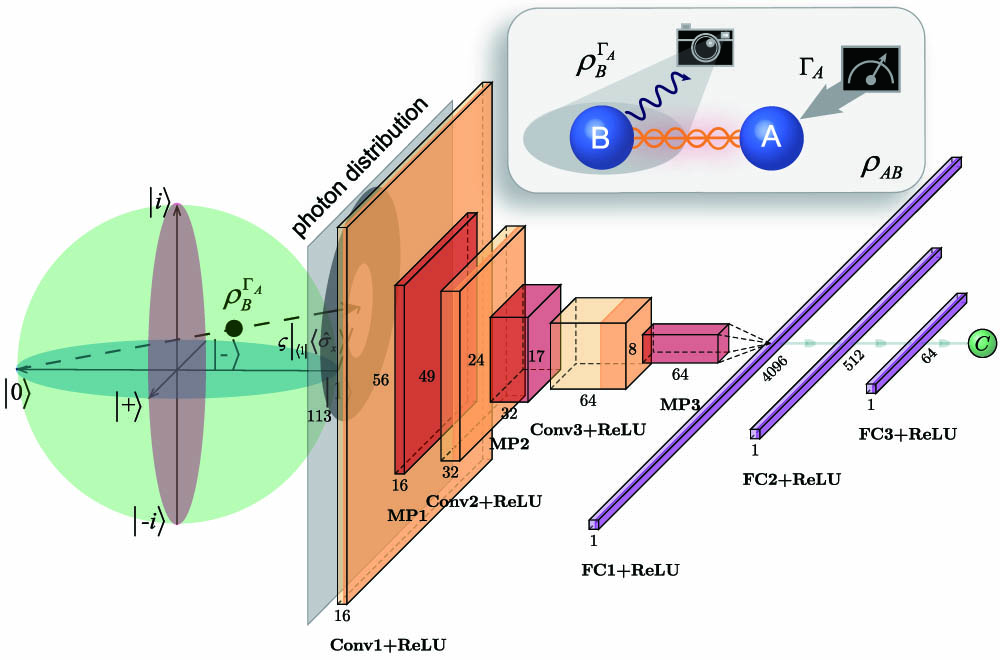
    Fig. 1. Theoretical framework and performance of the convolutional neural network (CNN). The weak values σ^x1|ΓAw and σ^x0|ΓAw of B on the state of ρBΓA (as shown in the Bloch sphere) are encoded in the central position of a Laguerre–Gaussian mode. The projected particle distribution is sent to the CNN to extract the concurrence. The boxes indicate the dimension (width of the box) and number (height of the box) of the feature maps. Convolution layers (Conv) with one stride are shown in a buff color. Activation functions (ReLU) of the convolution layers and full connection layers (FC) are denoted by the orange and purple colors, respectively. The red boxes indicate max-pooling layers (MPs) with two strides, and a small green ball represents the output concurrence. The arrows represent the flow of data. Insert: ρAB is a two-qubit entangled state. The spatial distribution of B’s conditional state ρBΓA is obtained, while a local projective measurement ΓA is performed on A.
    Experimental setup. (a) A pair of polarization-entangled photons are generated by pumping a type-II PPKTP crystal in a Sagnac interferometer with a 404 nm ultraviolet laser in the preparation stage. A half-wave plate HWP1 is set in front of the pump laser to rotate the polarizations. The polarizations of the pump light and down-converted photons are exchanged by the dual-wavelength HWP2, which is set to 45° in the Sagnac interferometer. HWP3 is used to change the form of the entangled state and is set to 45°. Bob’s and Alice’s photons pass through a weak measurement system (WM, shown in the gray dotted-line square) and an unbalanced interferometer (UI), respectively. The UI separates the photon into two paths by a beam splitter (BS). There are two sufficiently long calcite crystals (CCs) with the second length being twice larger than that of the first. In-between these crystals, HWP4 is set to 22.5° in one of the paths. This setup destroys the coherence in the different polarization components. Two variable filters (VFs, in the red dotted line circles) control the relative photon counts between the two arms. In the WM, the photon passes through a vortex phase plate (VPP, l=2) and is shaped into the Laguerre–Gaussian mode. HWP5, HWP6, and a thin birefringent crystal (TBC) with its axis set to 42° in the x-o-z plane are used to weakly couple the polarizations and momentum of the photon. (b) Quarter-wave plates (QWPs), HWPs, and polarization beam splitters (PBSs) on both sides of Alice and Bob (shown in the gray squares) are used to perform the projective measurements. On Bob’s side, the photons are detected by a single-photon detector (SPD) in the reflected path or by an intensified charge coupled device (ICCD) camera in the transmitted path. The signals detected by the SPD on Alice’s side are sent for coincidence or to trigger the ICCD camera. To train the convolutional neural network (CNN), the concurrence determined from the tomographic data is used as the label and the images recorded by the ICCD camera are used as the features, as indicated by the black and red arrows, respectively.
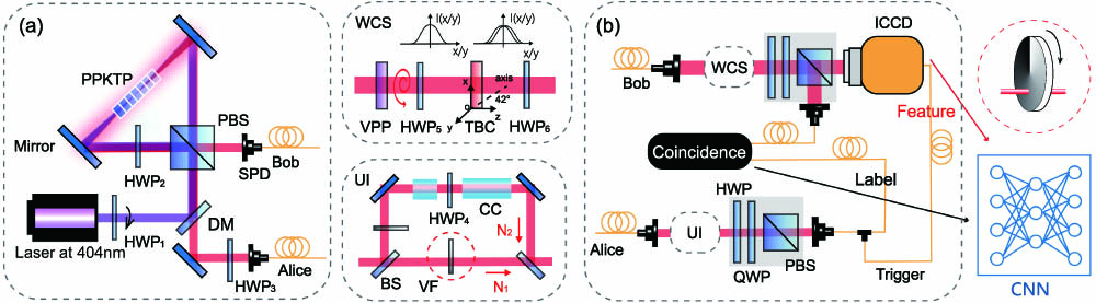
    Fig. 2. Experimental setup. (a) A pair of polarization-entangled photons are generated by pumping a type-II PPKTP crystal in a Sagnac interferometer with a 404 nm ultraviolet laser in the preparation stage. A half-wave plate HWP1 is set in front of the pump laser to rotate the polarizations. The polarizations of the pump light and down-converted photons are exchanged by the dual-wavelength HWP2, which is set to 45° in the Sagnac interferometer. HWP3 is used to change the form of the entangled state and is set to 45°. Bob’s and Alice’s photons pass through a weak measurement system (WM, shown in the gray dotted-line square) and an unbalanced interferometer (UI), respectively. The UI separates the photon into two paths by a beam splitter (BS). There are two sufficiently long calcite crystals (CCs) with the second length being twice larger than that of the first. In-between these crystals, HWP4 is set to 22.5° in one of the paths. This setup destroys the coherence in the different polarization components. Two variable filters (VFs, in the red dotted line circles) control the relative photon counts between the two arms. In the WM, the photon passes through a vortex phase plate (VPP, l=2) and is shaped into the Laguerre–Gaussian mode. HWP5, HWP6, and a thin birefringent crystal (TBC) with its axis set to 42° in the x-o-z plane are used to weakly couple the polarizations and momentum of the photon. (b) Quarter-wave plates (QWPs), HWPs, and polarization beam splitters (PBSs) on both sides of Alice and Bob (shown in the gray squares) are used to perform the projective measurements. On Bob’s side, the photons are detected by a single-photon detector (SPD) in the reflected path or by an intensified charge coupled device (ICCD) camera in the transmitted path. The signals detected by the SPD on Alice’s side are sent for coincidence or to trigger the ICCD camera. To train the convolutional neural network (CNN), the concurrence determined from the tomographic data is used as the label and the images recorded by the ICCD camera are used as the features, as indicated by the black and red arrows, respectively.
    Conditional states and photon spatial distributions. The numbered dots in the Bloch sphere represent the conditional projective states of Bob. Local photon distribution (IH) recorded by the ICCD camera with the corresponding concurrence (Cact) is shown in front of the Bloch sphere. The density matrix ρBΓA of the number 6 dot and the corresponding input state ρAB with p=0.9 and θ=0.81 are shown; here, the solid and transparent bars represent the experimental and theoretical results, respectively.
    Fig. 3. Conditional states and photon spatial distributions. The numbered dots in the Bloch sphere represent the conditional projective states of Bob. Local photon distribution (IH) recorded by the ICCD camera with the corresponding concurrence (Cact) is shown in front of the Bloch sphere. The density matrix ρBΓA of the number 6 dot and the corresponding input state ρAB with p=0.9 and θ=0.81 are shown; here, the solid and transparent bars represent the experimental and theoretical results, respectively.
    Experimental results. (a) CNN performance versus epoch. The brown curve represents the MSE value, and the green line represents the PCC between the actual concurrence Cacti and the predicted concurrence Cprei. (b) Distribution of predicted concurrences. The blue line represents the optimal curve. (c) Concurrence distributions in the p−θ space. The dots and contour lines represent the experimental and theoretical results, respectively. (d) Logarithm of MSE values of the entangled and separated states versus epoch. (e) CNN fivefold cross-validation performance. The result is averaged five folds. (f) CNN performance versus data size.
    Fig. 4. Experimental results. (a) CNN performance versus epoch. The brown curve represents the MSE value, and the green line represents the PCC between the actual concurrence Cacti and the predicted concurrence Cprei. (b) Distribution of predicted concurrences. The blue line represents the optimal curve. (c) Concurrence distributions in the pθ space. The dots and contour lines represent the experimental and theoretical results, respectively. (d) Logarithm of MSE values of the entangled and separated states versus epoch. (e) CNN fivefold cross-validation performance. The result is averaged five folds. (f) CNN performance versus data size.
    Value ⟨σ^x⟩⟨1|w of photon B on the state of ρBΓA is shown in the Bloch sphere, which is encoded in the photon B’s spatial distribution carrying orbital angular momentum.
    Fig. 5. Value σ^x1|w of photon B on the state of ρBΓA is shown in the Bloch sphere, which is encoded in the photon B’s spatial distribution carrying orbital angular momentum.
    Mu Yang, Ya Xiao, Ze-Yan Hao, Yu-Wei Liao, Jia-He Cao, Kai Sun, En-Hui Wang, Zheng-Hao Liu, Yutaka Shikano, Jin-Shi Xu, Chuan-Feng Li, Guang-Can Guo. Entanglement quantification via weak measurements assisted by deep learning[J]. Photonics Research, 2024, 12(4): 712
    Download Citation