【AIGC One Sentence Reading】:Utilizing weak measurements and deep learning, we've developed a method to directly detect entanglement in two-photon polarization-entangled mixed states, reducing the need for extensive projective bases compared to traditional quantum state tomography.
【AIGC Short Abstract】:Utilizing weak measurements enhanced by deep learning, this study introduces a method for directly detecting entanglement in two-photon polarization-entangled mixed states. This approach significantly reduces the need for extensive measurement data and estimation compared to quantum state tomography, simplifying the entanglement quantification process for mixed states.
Note: This section is automatically generated by AI . The website and platform operators shall not be liable for any commercial or legal consequences arising from your use of AI generated content on this website. Please be aware of this.
Abstract
Entanglement has been recognized as being crucial when implementing various quantum information tasks. Nevertheless, quantifying entanglement for an unknown quantum state requires nonphysical operations or post-processing measurement data. For example, evaluation methods via quantum state tomography require vast amounts of measurement data and likely estimation. Although a direct entanglement determination has been reported for the unknown pure state, it is still tricky for the mixed state. In this work, assisted by weak measurement and deep learning technology, we directly detect the entanglement (namely, the concurrence) of a class of two-photon polarization-entangled mixed states both theoretically and experimentally according to the local photon spatial distributions after weak measurement. In this way, the number of projective bases is much smaller than that required in quantum state tomography.
1. INTRODUCTION
Entanglement is an essential resource for nonclassical information tasks in quantum communication [1,2] and quantum computation [3,4], and has also been applied to nonlinear molecular spectroscopy [5]. However, quantifying entanglement requires nonphysical operations or post-processing of the measurement data [6].
One of the most common quantifications of entanglement is concurrence [7,8], and its determination generally requires quantum state tomography [9,10], which relies on projective measurements to form a set of projective bases on the Hilbert space of the system, providing all the information about the state. The number of projective bases increases exponentially with the system scaleup. When the scale of the system is very large, it is impossible to perform projective measurements. To circumvent this impossibility, several approaches have been proposed to quantify the concurrence, including collective measurements [11] and the interference between two copies of the quantum states [12]. However, such approaches contrapose two-qubit pure states and cannot be directly applied to the case of the complicated mixed state.
Recently, weak measurement technology has been used to directly detect quantum states, including the transverse wavefunction of the photon states [13], the density of a mixed two-qubit state [14], and even entangled states [15]. The weak measurement can extract a small amount of information from a single outcome. Although each outcome of the weak measurement is uncertain, the average value can build a certain value, named weak value, to reveal the state information.
Sign up for Photonics Research TOC. Get the latest issue of Photonics Research delivered right to you!Sign up now
In this study, we experimentally use the wake values to demonstrate the feasibility of entanglement quantification associated with a deep learning two-photon polarization-entangled system. Specifically, we compress the weak value information of two-qubit photonic states into local conditional states, which are illustrated via the spatial distributions of photons. An end-to-end relationship between the concurrence and the distribution of photons is determined by a well-trained convolutional neural network (CNN) [16]. We find that only two projective bases are needed to predict the concurrence, greatly reducing the operation time. Besides, the generalization of this method can quantify the entanglement of high-dimensional multiparticle pure states, and the advantage of this method is exponentially increased.
2. THEORETICAL FRAMEWORK AND CNN PERFORMANCE
Here, we consider a two-qubit (A and B) system, which is in a class of quantum states as [17] where and . and are two state parameters. These states are of the form X-type, and the parameter controls the components of pure states and mixed states. Figure 1 (insert) shows the main processes involved in our approach, in which we perform a local projective measurement on A, where . The information about entanglement is compressed into the local conditional state of B, written as To extract the information about entanglement, one can execute a weak measurement of the Pauli observable on B [18,19]. Via post-selecting on the state (), the obtained weak value [20,21] can be written as which is closely related to the density matrix elements of . This value reflects the distance between and the maximally mixed state , which is visually illustrated in the Bloch sphere in Fig. 1 (see Appendixes A and B for more details). The concurrence of the class states can be expressed as In particular, when is the pure state, is reduced to , and is reduced to identity measurement [7].
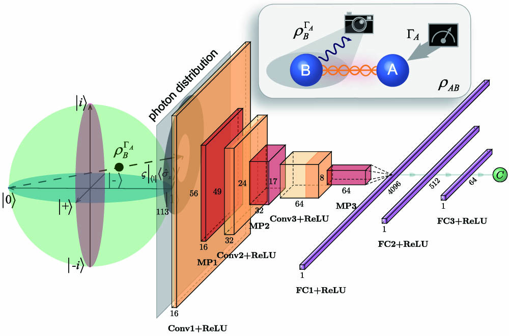
Figure 1.Theoretical framework and performance of the convolutional neural network (CNN). The weak values and of B on the state of (as shown in the Bloch sphere) are encoded in the central position of a Laguerre–Gaussian mode. The projected particle distribution is sent to the CNN to extract the concurrence. The boxes indicate the dimension (width of the box) and number (height of the box) of the feature maps. Convolution layers (Conv) with one stride are shown in a buff color. Activation functions (ReLU) of the convolution layers and full connection layers (FC) are denoted by the orange and purple colors, respectively. The red boxes indicate max-pooling layers (MPs) with two strides, and a small green ball represents the output concurrence. The arrows represent the flow of data. Insert: is a two-qubit entangled state. The spatial distribution of B’s conditional state is obtained, while a local projective measurement is performed on A.
To conveniently access the weak values, here we introduce orbital angular momentum (OAM) as a pointer, where the real and imaginary parts of are encoded as the coordinate - and -positions, respectively, of the central singular point [18,19] of the Laguerre–Gaussian (LG) mode on the local spatial distribution (see Appendix C for more details). This singular center can be extracted by straightforward optimal estimation or the least-square fit method. However, this weak shifting of the singular center is too susceptible to be effectively identified because of the experimental noise. To solve this problem, we attempt to directly extract the concurrence from the local spatial distribution by using a deep learning (DL) method [22], which has been used to solve many-body [23], large-scale quantum tomography [24], quantum state [25], and nonclassical correlation [26] problems. Specifically, we use a CNN to establish end-to-end mapping from the photon distribution to the concurrence, which avoids taking account of the form of the fitting functions or the relations between the weak values and concurrence. To train the CNN, we prepare a large number of two-qubit states . The corresponding local spatial distributions are used as features, and the concurrences determined from the tomographic data are used as the label. After being trained with a substantial number of distribution-concurrence pairs, the CNN establishes a statistical functional mapping between the local spatial distributions and the concurrence. The concurrence of the training set is labeled using the traditional method [7,8] by reconstructing the density matrix . The CNN also considers the imperfection of the local spatial distribution, so this method has high accuracy and strong robustness.
As shown in Fig. 1, the CNN consists of two paths: the convolution path and the full connection (FC) path. There are three blocks in the convolution path. The input images are mapped into the feature space by convolution layers and downsampled by max-pooling layers to magnify the weak variance in each block. To fit the concurrence, the output results of the convolution path are flattened into a one-dimensional vector and sent to the FC path, which contains four layers with different neurons. The activation function of each layer is selected to be ReLU [] so that the network can fit the nonlinear function. We use the Adam optimizer [27], which can effectively prevent local optimization. The mean squared error (MSE), which is used as the loss function, is defined as , where is the total number of samples, represents the actual concurrence labeled by the traditional method, and means the predicted concurrence. Some neurons were deleted to prevent overfitting (see Appendix D for more details).
3. EXPERIMENTAL DEMONSTRATION
The experimental setup is shown in Fig. 2. A 20 mm long periodic (PPKTP) crystal located in the Sagnac interferometer [28] is pumped by a 404 nm continuous-wave diode laser to create a pair of polarization-entangled photons via a type-II spontaneous parametric down-conversion process. These two photons are then sent to Alice and Bob. To generate the entangled state (where and represent horizontal and vertical polarization, respectively), a half-wave plate is used to control the parameter by rotating the polarization of the pump laser.
Figure 2.Experimental setup. (a) A pair of polarization-entangled photons are generated by pumping a type-II PPKTP crystal in a Sagnac interferometer with a 404 nm ultraviolet laser in the preparation stage. A half-wave plate is set in front of the pump laser to rotate the polarizations. The polarizations of the pump light and down-converted photons are exchanged by the dual-wavelength , which is set to 45° in the Sagnac interferometer. is used to change the form of the entangled state and is set to 45°. Bob’s and Alice’s photons pass through a weak measurement system (WM, shown in the gray dotted-line square) and an unbalanced interferometer (UI), respectively. The UI separates the photon into two paths by a beam splitter (BS). There are two sufficiently long calcite crystals (CCs) with the second length being twice larger than that of the first. In-between these crystals, is set to 22.5° in one of the paths. This setup destroys the coherence in the different polarization components. Two variable filters (VFs, in the red dotted line circles) control the relative photon counts between the two arms. In the WM, the photon passes through a vortex phase plate (VPP, ) and is shaped into the Laguerre–Gaussian mode. , , and a thin birefringent crystal (TBC) with its axis set to 42° in the x-o-z plane are used to weakly couple the polarizations and momentum of the photon. (b) Quarter-wave plates (QWPs), HWPs, and polarization beam splitters (PBSs) on both sides of Alice and Bob (shown in the gray squares) are used to perform the projective measurements. On Bob’s side, the photons are detected by a single-photon detector (SPD) in the reflected path or by an intensified charge coupled device (ICCD) camera in the transmitted path. The signals detected by the SPD on Alice’s side are sent for coincidence or to trigger the ICCD camera. To train the convolutional neural network (CNN), the concurrence determined from the tomographic data is used as the label and the images recorded by the ICCD camera are used as the features, as indicated by the black and red arrows, respectively.
On Alice’s side, the photon beam passes through an unbalanced interferometer (UI), first separated into two paths by a beam splitter (BS). Two sufficiently long calcite crystals (CCs) with set to 22.5° between them are placed on one of the paths to destroy the coherence between the different polarization components. In contrast, the state in the other path remains unchanged. Two variable filters (VFs) are used to change the relative photon counts in these two paths ( and ), where the parameter can be written as . The two-qubit states can be prepared when these two paths are combined.
On Bob’s side, the photon passes through a weak coupling system (WCS). A vortex phase plate (VPP) is placed to generate an LG wavefunction with an OAM of . Thereafter, a thin calcite crystal (TBC) with a thickness of 0.7 mm is employed to introduce a weak interaction between the polarization and the momentum of the photon; its optical axis is set in the plane, and it is oriented at 42° with respect to the axis [29]. Combining a pair of HWPs ( and ) with optical axes set to 22.5°, the interaction Hamiltonian is , where represents the momentum operator, is the coupling strength, and .
The polarization states on both sides are measured by a group of quarter-wave plates (QWPs), an HWP, and a polarization beam splitter (PBS). The coincidence from tomographic measurement is used as the label of CNN while the photon distributions are used as the input features of CNN. On Alice’s side, the photon is detected by a single-photon detector (SPD), and the signal is sent for coincidence or to trigger the intensified charge-coupled device (ICCD) camera on Bob’s side. In our experiment, we use a coincidence window of 3 ns and an exposure time of 1 s for all measurements. The projective direction on Alice’s side only needed to be selected as () in this experiment.
On Bob’s side, the photon is detected by an SPD and an ICCD camera in the reflected path and the transmitted path, respectively. The signal from SPD is sent for coincidence to reconstruct the experimental density matrix (the reflected path of the PBS). The fidelities between the theoretical physical states and the experimental states are more than 92%. The concurrences are calculated from [7,8]. The photon spatial distributions are detected by the ICCD camera. A small down-rightward deflection (; see Appendix C for more details) is introduced [18,19] after post-selecting the photon state onto the basis (). can be obtained according to Eq. (3) with representing the corresponding local conditional state. The final intensities and of the photon spatial distributions are detected by the ICCD camera (Fig. 3). Obviously, only a single projective base is needed to detect the weak value while quantum state tomography (QST) needs 16 projective bases. The total number of photon pairs that contribute to each base is approximately 600,000 (600,000 repetitions) with integral time 1 s. If the number of repetitions is too small, the estimation error will be increased, and more data will be required to train the CNN.
Figure 3.Conditional states and photon spatial distributions. The numbered dots in the Bloch sphere represent the conditional projective states of Bob. Local photon distribution () recorded by the ICCD camera with the corresponding concurrence () is shown in front of the Bloch sphere. The density matrix of the number 6 dot and the corresponding input state with and are shown; here, the solid and transparent bars represent the experimental and theoretical results, respectively.
In our experiment, we prepared 415 states, with 349 of the feature-label pairs being randomly chosen to be in the training data and the remaining 66 pairs serving as test data. Some photon distributions with different concurrences in the training set and an example of matrices and are shown in Fig. 3.
We first investigated the convergence of CNN. The performance with training time (epoch) is shown in Fig. 4(a). The weight of the CNN is optimized with the batch size 10 for 200 epochs. MSE (brown line) falls below 0.07 and PCC (green line) reaches 0.92 at the end of the training process, which demonstrates small prediction errors and strong relevance. The CNN learns more and more information concerning the entanglement with increasing epochs and is well trained when the epoch number is 200.
Figure 4.Experimental results. (a) CNN performance versus epoch. The brown curve represents the MSE value, and the green line represents the PCC between the actual concurrence and the predicted concurrence . (b) Distribution of predicted concurrences. The blue line represents the optimal curve. (c) Concurrence distributions in the space. The dots and contour lines represent the experimental and theoretical results, respectively. (d) Logarithm of MSE values of the entangled and separated states versus epoch. (e) CNN fivefold cross-validation performance. The result is averaged five folds. (f) CNN performance versus data size.
To demonstrate the predicted concurrence () accuracy of the trained CNN, we compared it to the concurrence (actual concurrence ) calculated by QST. The predicted concurrences (brown dots) for the test data are shown in Fig. 4(b). The point distribution is close to the optimal curve (blue line), which means that the predicted concurrences approximate the actual concurrences. We can also find the errors (uncertainty) between the concurrence predicted by CNN and the actual concurrence is less than 0.2 (). With further optimization of the CNN parameters and an increase in the training data, the error can be further reduced.
The predicted concurrence distributions in the parameter space of are shown in Fig. 4(c). The contour lines represent the theoretical boundaries of , and the predicted concurrence agrees with the theoretical trend. The values of the dots are calculated by minimizing the value of . We further investigated the source of the error shown in Fig. 4(d). With an increase in the training time, the average MSE of the separable states in the test set approaches (red bars), while the average MSE of the entangled states in the test set approaches (blue bars); these values are reached when epoch is greater than 160. These results imply that the CNN is more accurate when determining separated states.
To estimate how the model is expected to perform in general cases with limited samples, a fivefold cross-validation was implemented with our CNN. The data set was split into five parts, and each part was chosen in turn to be the test set, while the rest were used as the training set sent to the CNN. The mean MSE and PCC values of all five results converged to 0.09 and 0.87, respectively, when the epoch number is 200, as shown in Fig. 4(e).
Figure 4(f) demonstrates that the result is dependent on the amount of data. With an increasing data size, we should be able to predict the entanglement with greater accuracy.
4. SCALABILITY
It is worth noting that our entanglement quantification method remains efficient even when scaling to pure states with larger numbers of qubits or higher dimensions. To illustrate this, we present the results of three-qubit pure states and two-qutrit pure states below. The concurrence for multipartite pure states in arbitrary dimensions can be expressed as [30] where represents the set of all possible bipartitions of , and is the reduced density matrix across these bipartitions.
For three-qubit states , there are three possible bipartitions: , , . The concurrence of an arbitrary three-qubit pure state can be rewritten as , , where , , and represent the measurement on the corresponding subsystem (, ), (, ), and (, ), respectively. Clearly, using the weak measurement method, only three projective bases are required to quantify the entanglement of any three-qubit pure state. However, 64 projective bases are required for tomography.
In the computational basis , an arbitrary two-qutrit pure state can be expressed as
By combining Eq. (5) and Eq. (6), we can obtain , where represents the reduced density matrix of Bob in the qubit subsystem. is the matrix element of in the -th row and -th column, where and . Furthermore, it can be easily demonstrated that , where , and represents the identity measurement. Clearly, for any two-qutrit pure state, only three projective bases are needed to quantify the entanglement. However, when employing tomography, 81 projective bases are required.
As for universal N-partite D-dimensional pure state, there are possible bipartitions and possible qubit subsystems; thus, no more than projective bases are needed to quantify the entanglement. represents round down to the nearest integer, and represents the number of all combinations of taking distinct elements from distinct elements. In contrast, tomography requires projective bases. Clearly, the benefits of our method become increasingly apparent as the scale and the number of dimensions of the system increase.
5. CONCLUSION AND DISCUSSION
In this study, we established the relations between the concurrence and weak values, where the weak values were encoded into the transverse Laguerre–Gaussian (LG) photon distributions. By detecting the shift of singular center, we can directly get the concurrence. This weak measurement method will greatly reduce the number of projective bases and save the measurement resources. For a class of mixed two-qubit states, two projective bases are sufficient to quantify the entanglement, while 16 bases are required for tomography. Assisted by the DL method, we can achieve an “end-to-end” mapping between the photon distribution and concurrence without considering the form of the mapping functions. Moreover, this method, which takes the whole photon distribution as the input, can avoid estimation errors because it extracts the singular center weak shift.
We also show that the advantages of our method become more pronounced when scaling to larger numbers of qubits or higher dimensions, which demonstrates that our entanglement quantization method exhibits increasingly evident advantages over quantum state tomography as the system scales up. This highlights the potential of our method to efficiently characterize entanglement in large-scale quantum systems.
Acknowledgment
Acknowledgment. This work was supported by the Innovation Program for Quantum Science and Technology (2021ZD0301400 and 2021ZD0301200), the National Natural Science Foundation of China (61725504, 11821404, and U19A2075), and the Anhui Initiative in Quantum Information Technologies (AHY060300). M. Yang is supported by the Postdoctoral Innovative Talents Support Program (BX20230349) and the Fundamental Research Funds for the Central Universities (WK2030000085). Y. Shikano is supported by JSPS KAKENHI (17K05082, 18KK0079, and 19H05156) and JST PRESTO (JPMJPR20M4). Y. Xiao is supported by the National Natural Science Foundation of China (12004358), the Fundamental Research Funds for the Central Universities (202041012 and 841912027), the Natural Science Foundation of Shandong Province of China (ZR2021ZD19), and the Young Talents Project at Ocean University of China (861901013107).
APPENDIX A: RELATIONSHIP BETWEEN CONDITIONAL STATE ρBΓA AND THE VALUES ?σ^x?w?0(1)|
For a two-qubit system , the local conditional state can be generally represented as The weak values of with the post-selected state being and are, respectively, denoted as For any physical state, and . The elements of the density matrix can be expressed by which are determined by these two weak values. In our work, CNN needs only original information. The photon distribution on Bob’s side with the post-selected state and is used as the input feature.
APPENDIX B: REPRESENTATION OF THE VALUES |?σ^x??1|w| IN THE BLOCH SPHERE
It is well known that the conditional state of can be expressed as where and . indicates the position of the conditional state of in spherical coordinates. As shown in Fig. 5, the connection between the pure state and intersects with the x-o-y plane. Obviously, the distance between these intersected points and the center of the sphere (corresponding to maximally mixed state ) is It is worth noting that is related to the distance between the conditional state and maximally mixed state .
Figure 5.Value of photon B on the state of is shown in the Bloch sphere, which is encoded in the photon B’s spatial distribution carrying orbital angular momentum.
According to Eq. (A2), the values can be expressed as As a result, the value reflects the distance between the conditional state and maximally mixed state . In addition, the representation of the weak value is similar to .
APPENDIX C: WEAK VALUE EXTRACTION FROM THE CONDITIONAL SPATIAL DISTRIBUTIONS
For a two-qubit system , the local conditional state can be generally represented as The weak value of with the post-selected state () is denoted as Note that this definition can be taken as the formal formalism of the density-operator-based weak value [31]. In our experiment, and the transverse field are chosen to be the system and the pointer, respectively. The whole density matrix is After weak coupling, described by the interaction Hamiltonian , the whole system is obtained as where (assuming ). By post-selecting the system on the state , we get the pointer state Taking Eq. (C2) into the pointer state, the pointer state becomes For the LG beam , the pointer state satisfies Therefore, the weak value information is encoded into the pointer state and detected by ICCD as conditional spatial distributions [32,33]. The differentiation due to the approximation was discussed in Ref. [34].
APPENDIX D: MECHANISM OF THE CNN
In the convolutional (Conv) path, the matrix of input image is transferred into a feature space through three convolutional-max pooling layers. To illustrate the convolution operation, assume that the filter of the Conv layer is The output feature matrix is denoted as where , represent the element indices of the matrix. To reduce the size of feature space, a max pooling (MP) layer is set followed by the Conv layer. Assuming the filter of the MP layer is , the output matrix can be written as By implementing the same operations three times, the Conv path would output the final feature map, which is flattened into a one-dimensional vector and sent to full connection (FC) layers. The FC consists of four layers, which is constructed through the relation and represent the weight matrix and bias, respectively, which would be updated in the training process. The nonlinear function ReLU is defined by . The output is compared with the actual concurrence. The errors are sent back to the networks to optimize the weight matrix and bias .
 AI Video Guide
  AI Picture Guide
 AI One Sentence