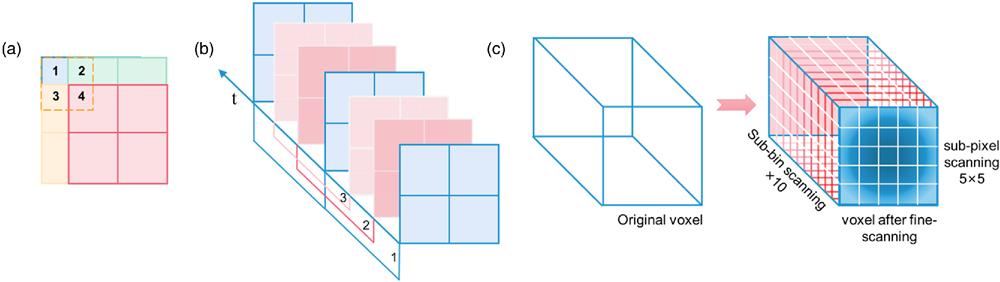
Fig. 1. Schematic of the 3D sub-voxel scanning method. (a) An illustration of sub-pixel scanning using the SPAD array with 2 pixel × 2 pixel and an inter-pixel spacing of 1/2 FoV. (b) A scheme of sub-bin scanning in time domain with 3 steps. (c) One original voxel in the measurement matrix can be expanded to 5×5×10 sub-voxels after fine scanning.

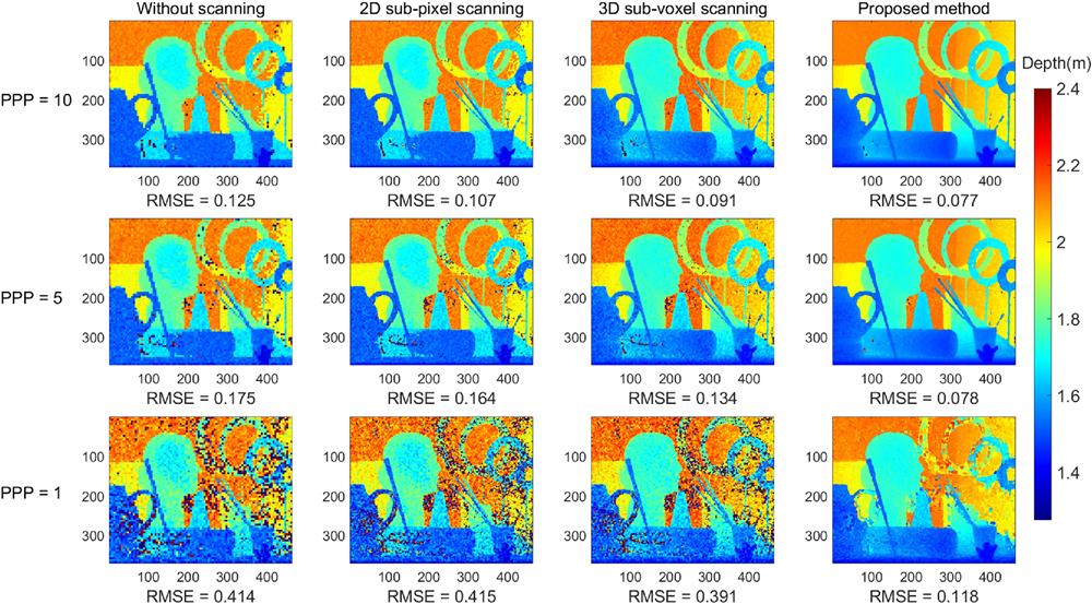
Fig. 2. Numerical simulation of the proposed algorithm. The ground truth is a typical scene from the Middlebury dataset. In our simulation, the SBR is set to 0.2, and the average number of detected signal photons is set to 10, 5, and 1 PPP, respectively. The first column shows the results without fine scanning. The second column shows the results with only 2D sub-pixel scanning and conventional pixel-wise ML processing. The third column shows the results with 3D sub-voxel scanning and pixel-wise ML processing. The last column shows the results with 3D sub-voxel scanning and our photon-efficient 3D deconvolutional algorithm. Quantitative results in terms of the RMSE are shown at the bottom of each figure. Clearly, our 3D sub-voxel method combined with the proposed algorithm has a smaller RMSE and superior performance to exhibit the details of the images.

Fig. 3. Schematic diagram of the experimental setup. (a) The schematic diagram of our experimental setup. The complex scenario is hidden behind a double-layer camouflage net, which is imaged by a visible-light camera, a MWIR camera, and our single-photon LiDAR system. (b) The photograph of the hidden scene. (c) The photograph of our experimental setup. (d) The photograph during the experiment with the glass door closed as an obstruction in the imaging path.

Fig. 4. Calibration results of our imaging system. (a) The calibration result of the PSF2D including 5 pixel × 5 pixel. (b) The calibration result of Box(t)*IRF(t). The red line is the Gaussian fit of the raw data. (c) The 3D model of the resolution chart. (d) The results are captured by single-photon LiDAR without fine scanning, with 2D sub-pixel scanning, and with 3D sub-voxel scanning, respectively.

Fig. 5. Experimental results of the static scenario behind the camouflage nets in daylight. The results of the (a) visible-light camera, (b) MWIR camera, (c) single-photon LiDAR without fine scanning, (d) single-photon LiDAR with 3D sub-voxel scanning, and (e) timing histogram of the data in (d).

Fig. 6. Experimental results of the static scenario behind the camouflage nets in daylight with a glass door. The results of the (a) visible-light camera, (b) MWIR camera, (c) single-photon LiDAR without fine scanning, and (d) single-photon LiDAR with 3D sub-voxel scanning. (a) and (b) are applied with contrast enhancement for better visual effects.

Fig. 7. Experimental results of the static scenario behind the camouflage nets at night. The results of the (a) visible-light camera, (b) MWIR camera, (c) single-photon LiDAR without fine scanning, and (d) single-photon LiDAR with 3D sub-voxel scanning. (a) and (b) are applied with contrast enhancement for better visual effects.

Fig. 8. Experimental results of the moving scenario behind the camouflage nets. (a) The photographs of the scene behind the camouflage nets taken from the back. (b) The photographs are captured by a MWIR camera. (c) The photographs are captured by a visible-light camera. (d) The reconstructed 3D profile of the multi-layer scenario. The movement of the mannequin and the basketball can be seen in the image sequences. The boxes of different colors indicate the segmented objects in our experiment.

Fig. 9. Comparison of 3D reconstruction methods for moving targets behind the camouflage nets. The data are the same as the first frame displayed in Fig. 8. Reconstruction results of the (a) cross-correlation, (b) real-time plug-and-play denoiser^[15], and (c) proposed method.

Table 1. Motion compensation algorithm