Highly efficient nonuniform finite difference method for three-dimensional electrically stimulated liquid crystal photonic devices

Zhenghao Guo; Mengjun Liu; Zijia Chen; Ruizhi Yang; Peiyun Li; Haixia Da; Dong Yuan; Guofu Zhou; Lingling Shui; Huapeng Ye

doi:10.1364/PRJ.516364

Abstract

Liquid crystal (LC) photonic devices have attracted intensive attention in recent decades, due to the merits of tunability, cost-effectiveness, and high efficiency. However, the precise and efficient simulation of large-scale three-dimensional electrically stimulated LC photonic devices remains challenging and resource consuming. Here we report a straightforward nonuniform finite difference method (NFDM) for efficiently simulating large-scale LC photonic devices by employing a spatially nonuniform mesh grid. We show that the NFDM can be further accelerated by approximately 504 times by using the improved successive over-relaxation method (by 12 times), the symmetric boundary (by 4 times), the momentum gradient descent algorithm (by 3.5 times), and the multigrid (by 3 times). We experimentally fabricated the large-scale electrically stimulated LC photonic device, and the measured results demonstrate the effectiveness and validity of the proposed NFDM. The NFDM allocates more grids to the core area with steep electric field gradient, thus reducing the distortion of electric field and the truncation error of calculation, rendering it more precise than the finite element method and traditional finite difference method with similar computing resources. This study demonstrates an efficient and highly reliable method to simulate the large-scale electrically stimulated LC photonic device, and paves the way for customizing a large-scale LC photonic device with designable functionalities.

1. INTRODUCTION

Liquid crystals (LCs) are a kind of optically birefringent material with dielectric anisotropy, which can be denoted by two orthogonal principal axes, namely the short and long axes [1,2]. The long axis of LC molecules (positive liquid crystals) is consistent with its director direction, and is responsive to external stimuli such as electric field, heat, light, or surface molecular anchoring force [1 –4]. In principle, reorienting the director of LC molecules is equivalent to redefining the dynamic or geometric phase retardation brought by LCs, which facilitate vast applications ranging from optical sensor [5,6], head-mounted display [1,7,8], and spatial light modulator [9,10] to electrically tunable lens/microlens [2,11 –15] and special beam generator [16 –19]. Hence, obtaining the director configuration of LC molecules plays a vital role in numerically analyzing, simulating, and designing the LC photonic devices with multifarious functionalities.

So far, the simulation of the director configuration of large-scale LC photonic devices in the presence of both external stimulus and surface molecular anchoring force usually adopts coarse and uniform mesh grids to the LC layer, due to the limited computing resources and the large size of the device [20 –22]. This may induce uncertainty and cause serious error to the simulation in case of inhomogeneous and gradient stimulus, which leads to rapid directors morphing in certain regions such as the location of defects [23]. Hence, in order to obtain the accurate solution, it is noteworthy to allocate more computing resources to the critical region, implying that fine mesh should be employed to the area with dramatically changing directors. Meanwhile, in order to increase the efficiency, a relatively coarse mesh is sufficient for other regions with smoothly morphing directors. Generally, this task can be partially accomplished by using the finite element method (FEM), which flexibly meshes the model into triangular or tetrahedral elements. However, although FEM is widely considered as reliable method for calculating the two-dimensional LC director [24,25], it encounters difficulties when it is extended to the three-dimensional (3D) LC director, due to the computational resource-consuming procedures, including approximating the field variables of each element with an interpolating function and minimizing the residual of the differential equations [25]. The difficulty is further amplified when accurate director distribution should be obtained for light field simulation. By contrast, the traditional finite difference method (FDM), which meshes the model into uniform cuboid units, consumes far fewer resources than FEM [20,26]. However, in order to increase the accuracy of FDM, the grid size should be adjusted uniformly at the cost of increasing the computing resources exponentially and wasting resources in the low gradient region. Therefore, it remains challenging to simulate large-scale 3D LC photonic devices accurately, due to the limitation of computational resources and efficiency.

Herein we report a nonuniform finite difference method (NFDM) to efficiently simulate a large-scale 3D electrically stimulated LC photonic device with high accuracy via flexibly controlling the grid density in the area with steep spatial gradient stimulus. We accelerate the NFDM by approximately 504 times, via using a stepwise parallel successive over-relaxation (SOR) method (by 12 times), the symmetric boundary (by 4 times), the momentum gradient descent (MGD) algorithm (by 3.5 times), and the multigrid (by 3 times). Studies based on the finite difference time domain (FDTD) software prove that NFDM has higher stability and accuracy than the FEM and traditional FDM. The diffraction field of the LC device is efficiently simulated with low computing resources by combining the NFDM, the vectorial Rayleigh–Sommerfeld diffraction formula, and fast Fourier transform. Furthermore, we experimentally fabricated the large-scale electrically stimulated LC photonic device, and the measured results demonstrate the effectiveness and validity of our proposal. This study provides an efficient and accurate method to simulating the LC photonic device, which may facilitate the design and optimization of LC photonic devices with customized functionalities.

Sign up for Photonics Research TOC. Get the latest issue of Photonics Research delivered right to you！Sign up now

2. THEORY AND METHODS

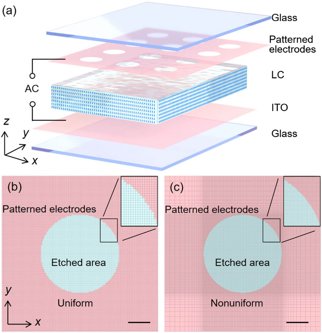
In order to explicitly illustrate our proposal, let us take the LC photonic device consisting of patterned electrode array [see Fig. 1(a)] for example. The LC device consists of two plane glasses with inner surface spin-coated with conductive indium tin oxide (ITO) film. One of the ITO films is patterned into the electrode array. The LCs are sandwiched between the two glasses and form a planar cell. After applying the alternating current (AC) to the electrodes, the LC director tends to assemble into a certain configuration in response to the electric field and then forms the LC lens consequently [11,12]. Figures 1(b) and 1(c) depict the mesh grid of the patterned electrodes by using uniform [Fig. 1(b)] and nonuniform [Fig. 1(c)] FDM with identical amounts of mesh grids. Evidently, the grid of the nonuniform method is finer than the uniform method in the etched area via allocating more grids to the core area with steep electric field gradient. The details of the simulation method of the LC director and the acceleration algorithms to increase the calculation speed of NFDM are introduced in the following section.

(a) Schematic diagram of electrically stimulated LC photonic device. (b), (c) Grids of patterned electrode meshing in similar number of model grids. (b) Uniform grids and (c) nonuniform grids. The scale bars in (b), (c) are 10 μm.

Figure 1.(a) Schematic diagram of electrically stimulated LC photonic device. (b), (c) Grids of patterned electrode meshing in similar number of model grids. (b) Uniform grids and (c) nonuniform grids. The scale bars in (b), (c) are 10 μm.

A. Q Tensor and Director Simulation

According to the Frank–Oseen model [27], the LC director can be described by using vector $n = (n_{1}, n_{2}, n_{3})$ . However, it should be bore in mind that using vector $n$ to describe LC director configurations has a theoretical imperfection. Unlike actual LC molecules, the vector angle between the two directors can be larger than 90°, especially when the vectors orient opposite to each other, but the realistic LC directors are identical with head–tail symmetry. It leads to infinite energy in the LC topology defect (discontinuity in director) region in simulation, which cannot exist stably in simulation and is inconsistent with the reality. Hence, the results of using the vector method to simulate the LC devices with complex electrodes or surface molecular anchoring are unreliable. To mitigate this challenge, here we propose to adopt Landau-de Gennes’s Q tensor [28] to represent the uniaxial LC, and the $Q$ is defined as follows [22,23,29,30]: $Q = S (n \otimes n - \frac{1}{3} I) = S (\begin{matrix} n_{1} n_{1} - 1 / 3 & n_{1} n_{2} & n_{1} n_{3} \\ n_{1} n_{2} & n_{2} n_{2} - 1 / 3 & n_{2} n_{3} \\ n_{3} n_{1} & n_{3} n_{2} & n_{3} n_{3} - 1 / 3 \end{matrix}),$ (1)where $I$ is the identity matrix, $S$ is the order parameter, and $Q_{i j}$ is used to denote the $i j$ th element of $Q$ . As $Q$ is a symmetric traceless matrix, it has six different elements, namely $Q_{11}$ , $Q_{22}$ , $Q_{33}$ , $Q_{12}$ , $Q_{13}$ , and $Q_{23}$ . The Q tensor can avoid the head–tail asymmetry problem because the same $Q$ is used for $n$ and $- n$ .

Here, we use the Q tensor [Eq. (1)] and the potential $U$ to represent the elastic free energy density $f_{d}$ [see Eq. (A1) in Appendix A] and the electric free energy density $f_{e}$ [see Eq. (A2) in Appendix A]. Hence, the total energy $F_{g}$ can be obtained by integrating the Gibbs free energy density $f_{g}$ over the volume, namely $F_{g} = \int f_{g} d v = \int f_{d} - f_{e} d v$ . The total energy is minimum when the LC director reaches an equilibrium state by the constant external field. Therefore, the final LC director configuration can be obtained by solving Euler–Lagrange equations with constraint $| n | = 1$ : $0 = - {[f_{g}]}_{U},$ (2a) $0 = - {[f_{g}]}_{n_{i}} + λ n_{i}, i \in {1, 2, 3},$ (2b)where $λ$ is a Lagrange multiplier to constrain $| n | = 1$ . Eq. (2a) is Gauss’s law, ${[f_{g}]}_{h} = \frac{\partial f_{g}}{\partial h} - \sum_{i = 1, 2, 3} \frac{d}{d ξ_{i}} \frac{\partial f_{g}}{\partial (\partial h / \partial ξ_{i})}, h \in {U, Q_{11}, Q_{12}, Q_{13}, Q_{22}, Q_{23}, Q_{33}},$ (3)and ${[f_{g}]}_{n_{i}} = \sum_{j = 1, 2, 3} {[f_{g}]}_{Q_{i j}} \frac{\partial Q_{i j}}{\partial n_{i}} = 2 S \sum_{j = 1, 2, 3} n_{j} {[f_{g}]}_{Q_{i j}}, i \in {1, 2, 3} .$ (4)Here, we propose to adopt the relaxation method based on dynamics to solve Eq. (2), which is widely considered as a stable method to calculate the LC director [20,23,30,31]. The equation of the relaxation method can be given as below: $γ \frac{\partial n_{i}}{\partial t} = - {[f_{g}]}_{n_{i}} + λ n_{i}, i \in {1, 2, 3},$ (5)where $γ$ is the viscosity coefficient, $t$ is the time variable, and $λ$ is the Lagrange multiplier ensuring that $n$ is a unit vector. The component $λ n_{i}$ can be removed via vector normalization in each iteration. Taking the time difference of Eq. (5), we have $\frac{\partial n_{i}}{\partial t} = \frac{Δ n_{i}}{Δ t} = \frac{n_{i}^{t + Δ t} - n_{i}^{t}}{Δ t}, i \in {1, 2, 3} .$ (6)

Therefore, the iteration formula of relaxation method can be finally derived as ${\tilde{n}}_{i}^{t + Δ t} = n_{i}^{t} - \frac{Δ t}{γ} {[f_{g}]}_{n_{i}}, n^{t + Δ t} = \frac{{\tilde{n}}^{t + Δ t}}{| {\tilde{n}}^{t + Δ t} |}, i \in {1, 2, 3},$ (7)where $n^{t}$ and $n^{t + Δ t}$ are the director configuration at the current time step and the next time step, respectively, and ${[f_{g}]}_{n_{i}}$ is a value that indicates the level of the directors deviating from the low energy state. In each iteration, the total energy is reduced by turning a tiny angle in the opposite direction in proportion to ${[f_{g}]}_{n_{i}}$ . At the beginning of the iteration, a random director is set to the LC device, and a proper $Δ t / γ$ is chosen. The director configuration of the next step is obtained based on the iteration with the random director. The total energy decreases continuously during the iterations, and the director configuration eventually converges to the equilibrium state.

By solving Eq. (2a), we can obtain the iterative equation of the potential U in the LC layer. In principle, the potential U is zero at infinity. However, we use $d U / d z = 0$ at $4 d$ away from the LC layer with the error $O (e^{- 4 d})$ to replace the infinity [31], where $d$ is the LC layer thickness. Moreover, for simplicity, Gauss’s law is used to solve the potential distribution in the isotropic glass and the electrodeless region of ITO interface, which are given as $\nabla \cdot D = 0$ , $D = ε_{glass} \cdot E$ , and $E = - \nabla U$ .

B. Nonuniform FDM

As introduced above, it is impossible to solve the analytical solution for complex LC models. Hence, discretization methods are demanded in solving the numerical solution. In the traditional FDM, the first and second derivatives required by numerical iteration in the relaxation method for each discrete points can be represented by the values of adjacent points [see Eq. (A3) in Appendix A], namely using central difference. The grids in the whole calculation area are uniform; hence the grid density cannot be flexibly adjusted. To overcome this challenge, we propose the nonuniform FDM to calculate the director configuration, where the inhomogeneous grids can be meshed according to the gradient of the external field.

In order to derive the nonuniform FDM, the differentiable function $f (x, y)$ at points $x = x_{0} - Δ x_{1}$ and $x = x_{0} + Δ x_{2}$ is first expanded according to the Taylor expansion: $f (x_{0} - Δ x_{1}) = f (x_{0}) - Δ x_{1} f_{x}^{'} (x_{0}) + \frac{Δ x_{1}^{2}}{2!} f_{x x}^{''} (x_{0}) + O (Δ x_{1}^{3}),$ (8a) $f (x_{0} + Δ x_{2}) = f (x_{0}) + Δ x_{2} f_{x}^{'} (x_{0}) + \frac{Δ x_{2}^{2}}{2!} f_{x x}^{''} (x_{0}) + O (Δ x_{2}^{3}),$ (8b)where $x_{1}$ and $x_{2}$ approach 0, and $O (Δ x_{1}^{3})$ and $O (Δ x_{2}^{3})$ are negligible. By solving the variables in Eq. (8), we can obtain the first-order and second-order differential equations in Eqs. (9a) and (9b). Moreover, we can get the second-order differential equation along the $x y$ direction by taking the derivative of $f_{x}^{'}$ along the $y$ direction, which is given by Eq. (9c): $f_{x}^{'} (x_{0}) \approx \frac{Δ x_{1}^{2} f (x_{0} + Δ x_{2}) - Δ x_{2}^{2} f (x_{0} - Δ x_{1}) + (Δ x_{2}^{2} - Δ x_{1}^{2}) f (x_{0})}{(Δ x_{1} + Δ x_{2}) Δ x_{1} Δ x_{2}},$ (9a) $f_{x x}^{''} (x_{0}) \approx \frac{2 [Δ x_{1} f (x_{0} + Δ x_{2}) + Δ x_{2} f (x_{0} - Δ x_{1}) - (Δ x_{1} + Δ x_{2}) f (x_{0})]}{(Δ x_{1} + Δ x_{2}) Δ x_{1} Δ x_{2}},$ (9b) $f_{x y}^{''} (x_{0}, y_{0}) \approx \frac{Δ y_{1}^{2} f_{x}^{'} (x_{0}, y_{0} + Δ y_{2}) - Δ y_{2}^{2} f_{x}^{'} (x_{0}, y_{0} - Δ y_{1}) + (Δ y_{2}^{2} - Δ y_{1}^{2}) f_{x}^{'} (x_{0}, y_{0})}{(Δ y_{1} + Δ y_{2}) Δ y_{1} Δ y_{2}} .$ (9c)

After substituting Eq. (9) into Eqs. (2a) and (7), we can obtain the iterative formula for the potential and the director at each point in the LC model. During the iteration process of these formulas, the director distribution of next moment is iterated from that of the current moment. It should be mentioned that the truncation error [induced by neglecting $O (Δ x^{3})$ ] exists in all the iterations; however, it will not be accumulated during the whole iterative process. We propose to realize the nonuniform mesh grids via controlling $Δ x$ , $Δ y$ , and $Δ z$ . In the simulation, the grid density of FDM can be adjusted freely according to the gradient of the spatial electric field or surface molecular anchoring to improve the simulation accuracy and meanwhile save computing resources. It should be emphasized that the nonuniform grid is transformed into the uniform grid, when $Δ x_{1} = Δ x_{2} = Δ x$ and $Δ y_{1} = Δ y_{2} = Δ y$ .

C. Accelerating Algorithm

Equations (1)–(12) describe the fundamental formula for numerically calculating the spatial distribution of the LC director under stimulus of external electric field by FDM. However, the speed of the calculation based on these equations is unsatisfactory. In this study, we propose to accelerate the simulation by using the four algorithms, as introduced below. In order to evaluate the performance of each accelerating algorithm, we use the simulation times between turning on the algorithm and turning off the algorithm to calculate the acceleration value. To be fair, the configuration of the computer used for all simulations in this article is the same (CPU, Intel i5-10400F 2.9 GHz; GPU, NVIDIA GTX 1650s; RAM, 16G). It is worth noting that the numerical value of the speed increase is based on the LC device and grids shown in this study, although it may slightly change in case of different LC devices.

First, we discuss the problems that arise in the potential, which is calculated alternately with the LC director. During the potential iterative calculation in our simulation, the convergence rate slows down sharply when the result is close to the stable solution, rendering the electric field calculation hard to reach equilibrium state. In order to overcome this challenge, the SOR method is adopted to accelerate the convergence speed by providing additional power. The equation of the SOR method is written as [31,32] $U^{t} = (1 - ω) U^{t - Δ t} + ω {\tilde{U}}^{t},$ (10)where $ω$ is the relaxation parameter, $1 < ω < 2$ . The result of Eq. (10) diverges when $ω \geq 2$ , while it is transformed into the Gauss–Seidel method when $ω = 1$ [33]. During each iteration, the potential calculated result ${\tilde{U}}^{t}$ is taken as the temporary result, and the final potential $U^{t}$ is obtained by using Eq. (10). Proper $ω$ is chosen to accelerate the simulation, and it is set to about 1.98 in our calculation.

However, when the SOR method is used to calculate alternately with the director iterative equation, the result is divergent. In order to illustrate the problem, let us take the two-dimensional model [Fig. 2(a)] for example. We need to use the director and potential values of the surrounding blue points to calculate the iterative value of the potential at the red point. At the beginning, we attempted to use the SOR method alternate calculation with director iterative equation; however, we found that the results are fluctuating and highly diverging when calculating red and blue points simultaneously. Hence, to take full advantage of the matrix operation, we propose a stepwise parallel SOR method suitable for director simulation of FDM. As shown in Fig. 2(b), the iteration values of all points of each color are stepwise calculated and updated in order of blue, red, yellow, and green. With this method, we can avoid calculating the iteration values of adjacent points in the same iteration. Moreover, it should be mentioned that this method can be flexibly extended to the 3D model if it is divided into eight steps for calculation. The calculation speed of the potential is improved by about 12 times in our simulation.

Figure 2.(a) Schematic diagram of calculation relation. (b) Calculation sequence of SOR. (c), (d) Schematic diagram of (c) periodic and (d) symmetric boundary conditions. (e) Boundary conditions at different $p$ values.

Apart from the improved parallel SOR method we proposed, the periodic boundary condition can also be used to save the computing resources, as shown in Fig. 2(c), where a unit is simulated instead of the entire array. Furthermore, when the unit element [Fig. 2(d)] has axial symmetry along the array direction, the computing resources in case of applying symmetric boundary condition are only 1/4 of that using the periodic boundary condition. Due to the complexity of the boundary cases using the Q tensor, we derive the following formula for a general description: $p_{i j, ξ_{k}} = (- 1)^{δ_{i k}} (- 1)^{δ_{j k}} c_{ξ_{k}}, i, j \in {1, 2, 3}, k \in {1, 2},$ (11)where coordinate $(ξ_{1}, ξ_{2}) = (x, y)$ denotes the Cartesian coordinate system; $δ_{i j}$ is Kronecker’s delta ( $δ_{i j} = 1$ , when $i = j$ ; otherwise $δ_{j k} = 0$ ); $c_{x}$ and $c_{y}$ are the boundary conditions we set in $x$ and $y$ directions ( $c = 0$ denotes periodic and $c = 1$ for symmetric boundary); and $P_{i j, x}$ and $P_{i j, y}$ are the boundary conditions of $Q_{i j}$ in $x$ and $y$ directions, as shown in Fig. 2(e) ( $p = 0$ is periodic boundary, $p = 1$ is symmetric boundary, and $p = - 1$ is antisymmetric boundary). Furthermore, the $z$ -direction symmetry format can be easily extended and applied when the upper and lower pattern electrodes are consistent. In our simulation, the calculation speed of the symmetric boundary is improved to four times faster than that of the periodic boundary.

Sequentially, we adopted the momentum gradient descent algorithm to accelerate the director morphing from a disordered state to an equilibrium state [20,34], as given below: $Δ n_{i}^{t} = - \frac{Δ t}{γ} {[f_{g}]}_{n_{i}} + β Δ n_{i}^{t - Δ t},$ (12)with $Δ n_{i}^{t} = n_{i}^{t + Δ t} - n_{i}^{t}, Δ n_{i}^{t - Δ t} = n_{i}^{t} - n_{i}^{t - Δ t}$ , $i \in {x, y, z}$ , where $Δ n^{t}$ and $Δ n^{t - Δ t}$ denote the director change of the current iteration and the previous iteration, respectively; $β$ is a value usually set between 0.8 and 0.9. Here, the director $n$ has to be normalized after each iteration, and $Δ n^{t - Δ t}$ records all previously updated values with exponentially reduced weight due to Eq. (12). Therefore, the MGD algorithm accumulates momentum during the downhill and improves the update speed, but it slows down when approaching stability. Alternatively, adjusting the $Δ t / γ$ term dynamically can also achieve the same effect as the MGD algorithm. Finally, the LC director calculation is accelerated up to about 3.5 times faster by using the MGD algorithm in our simulation.

Finally, we adopt the multigrid [21] to speed up the calculation. In principle, the multigrid method first uses a coarser grid to construct the model. After completing the iterative computation, a finer grid is built for further calculation. The initial value of the director and potential of the finer grid are interpolated from the calculation results of the coarser grid and satisfy the setting of the electric fields. The simulation is terminated until the grid satisfies the requirements. It is found that the multigrid in our simulations can speed up the computation by approximately three times.

3. RESULTS AND DISCUSSION

In order to verify our proposal, numerical simulations based on FEM and uniform and nonuniform FDMs are conducted to the same model [Fig. 3(a)], where the periodic boundary condition is applied. The parameters are set as follows: the ITO electrodes array with circular aperture has diameter of 50 μm and period of 100 μm, the LC layer thickness is 50 μm, the LC material is 5CB ( $K_{11} = 6.2$ pN, $K_{22} = 3.9$ pN, $K_{33} = 8.2$ pN [35], $ε_{⊥} = 7.0$ (1 kHz), $ε_{| |} = 18.5$ (1 kHz), $n_{e} = 1.6975$ (589 nm), $n_{o} = 1.5350$ (589 nm), $q_{0} = 0$ [36]), and an AC voltage of 1 kHz with 200 V is applied. The upper and lower boundaries of the LC layer are set as strong homeotropic anchoring (fix the director vertically), and a random director configuration is set to other LC molecules.

Figure 3.(a) Schematic illustration of the unit cell of the LC photonic device. (b)–(j) Slice diagrams of the calculated tilt angle of the directors. (b)–(d) FEM, (e)–(g) uniform FDM, and (h)–(j) nonuniform FDM. (b), (e), (h) Along $x$ direction where $x$ is sampled at 50, 55, 60, 65, 70, 75, 80, and 85 μm. (c), (f), (i) Along $z$ direction where $z$ is sampled at 30, 35, 40, 45, and 49.5 μm. (d), (g), (j) Zoomed-in image of tilt angle diagrams of the directors.

We first simulated the LC directors based on the FEM method with the commercially available COMSOL software [37]. The model [Fig. 3(a)] was built in COMSOL, where the variational weak-form equations of the total energy $F_{g}$ [see Eq. (A4) in the Appendix A] were put into COMSOL’s physical interface of weak-form partial differential equation, and the vector normalization similar to Eq. (7) was applied to the director. The relative error ( $< 0.01$ ) was set as the iteration termination condition. When the minimum element size is set to 1 μm, the generated domain elements are 105,847 in the LC layer, and 90,270 in the glass region (Table 1). The simulation ran for 53.3 min on a laptop (CPU, Intel i5-10400F 2.9 GHz; GPU, NVIDIA GTX 1650s; RAM, 16G), and the results of director are depicted in Figs. 3(b)–3(d), where slice diagrams of the tilt angle of the directors are plotted. The FEM method based on COMSOL can directly lead to the solution after iteration and without using the relaxation method. However, the prominent mosaic effect existing in the zoomed-in image reveals that the directors based on FEM are not accurate. A more reliable method is demanded in this kind of simulation. More details about the FEM mesh can be found in Appendix B.Table 1.

Calculation Information of Three Methods

Methods	Minimum Element Size (μm)	Number of Domain Elements (LC Region)	Computational Resources (Gb)	Number of Iterations	Simulation Time (min)	Total Energy $F_{g}$ (J)
FEM (COMSOL)	1	105,847	13.6	11	53.3	$- 6.22 \times 10^{- 10}$
Uniform FDM	$0.69 \times 0.69 \times 0.48$	2,198,016	3.1	1253	7.4	$- 6.33 \times 10^{- 10}$
Nonuniform FDM	$0.29 \times 0.29 \times 0.3$	2,164,032	3.1	1551	10.2	$- 6.36 \times 10^{- 10}$
Uniform FDM (fine)	$0.3 \times 0.3 \times 0.31$	18,063,360	4.2	1955	45.1	$- 6.36 \times 10^{- 10}$

Next, we used the same computer and MATLAB software [38] to implement the uniform and nonuniform FDMs (described in Section 2.B) and simulate the LC directors of the same model for the purpose of comparison. The minimum grid sizes are set as $x \times y \times z = 0.69 μm \times 0.69 μm \times 0.48 μm$ in uniform FDM and $x \times y \times z = 0.29 μm \times 0.29 μm \times 0.3 μm$ in nonuniform FDM (Table 1). The design procedure of the nonuniform grid is to first use a coarse uniform grid for simulation to obtain the preliminary result, which is then used as basis to set up nonuniform grids. After the area and grid size of the fine grid are chosen, we determine the area and grid size of the coarse grid. Subsequently, we adopt a grid transition with a geometric sequence of sizes between the fine grid and the coarse grid in the simulation. The total mesh grids of LC directors are estimated to be $x \times y \times z = 144 \times 144 \times 106 = 2,198,016$ in uniform FDM and $x \times y \times z = 204 \times 204 \times 52 = 2,164,032$ in nonuniform FDM, respectively. We also performed comparison of FDM and NFDM with similar smallest spatial resolution (the results in the bottom row of Table 1). It can be seen that a fine FDM requires nine times the number of original grids, and the calculation time is significantly increased, ultimately achieving the same effect as NFDM. This directly proves the effectiveness of our method. In order to satisfy approximately zero potential at infinity with $d U / d z = 0$ ( $4 d$ away from the LC layer), the grids of the potential inside the glass substrate should be increased to four times of the director grids, as is necessary for calculating the electric field inside the glass. Moreover, the total energy of the system during the iterative calculation of the relaxation method is employed to denote the stability of the temporary LC director configuration. If the maximum change in the LC directors $n$ and potential $U$ between two iterations at all points satisfy ${(Δ n)}_{\max} < 5 \times 10^{- 7}$ (three components) and ${(Δ U)}_{\max} / U_{external} < 5 \times 10^{- 7}$ , where $U_{external}$ is the applied voltage, we consider the LC director field to reach an equilibrium state and shut off the iteration. When symmetric boundary conditions are employed, the simulation time of uniform and nonuniform FDM method is 7.4 min and 10.2 min (Table 1), respectively. It can be seen from Figs. 3(e)–3(j) that the LC directors lie almost planar at the edges, due to a strong in-plane component of electric field arising from the transverse electric field gradient. In principle, this gradient can be explained by the lower potential formed at the center of the etching area due to the lower surface electrode and the zero potential at infinity. Moreover, the simulated tilt angles of the LC directors in case of the uniform and nonuniform FDM are shown in Figs. 3(e)–3(j). It can be seen that the tilt angle distributions of the three methods are the same as each other both along the $x$ direction [Figs. 3(b), 3(e), and 3(h)] and the $z$ direction [Figs. 3(c), 3(f), and 3(i)]. However, according to the value of the lowest total energy $F_{g}$ (equilibrium state) in Table 1, it is reasonable to conclude that the nonuniform FDM generates better results than FEM and uniform FDM. Moreover, a significant difference exists and can be identified in the zoomed-in image [Figs. 3(d), 3(g), and 3(j)], which clearly indicates that the nonuniform FDM is most refined [Fig. 3(j)] and precise (lowest total energy).

The calculation information of the three methods (Table 1) illustrates that FEM uses far fewer domain elements than FDM; however, it consumes more computational time and resources. FEM uses an interpolation function to represent the distribution of director in the domain elements, but it cannot get accurate results due to the limitation of the number of elements and computational resources. Therefore, using FEM to simulate LC devices is inefficient and becomes challenging in the case of large-size devices. As a comparison, FDM leads to a similar result to FEM while consuming fewer resources and time (both less than a quarter). Moreover, nonuniform FDM takes slightly more time to calculate than uniform FDM, but yields finer results, which is acceptable. These results demonstrate the effectiveness of using nonuniform FDM to calculate the LC director configuration, which render it possible to simulate large-scale 3D LC devices. Moreover, compared with FEM, which solves the equation directly, nonuniform FDM using the pseudo-dynamic relaxation method is helpful to understand the LC behavior.

Figures 4(a)–4(c) plot the normalized grid density distribution of the nonuniform FDM in the $x z$ plane and $x y$ plane, which is described by $1 / (Δ x \times Δ y \times Δ z)$ . It can be observed that the mesh near the electrode is densest, and it gets sparse away from the electrode. This trend is clearly shown and confirmed by the zoomed-in image [Fig. 4(c)] and the red dashed curves in Figs. 4(d) and 4(e), where the grid sizes of the uniform and nonuniform methods are plotted. As the gradient of the electric field changes sharply near the electrode, thus inducing dramatic change to the director orientation, it is reasonable to allocate more mesh grids (smaller grid size) in these regions while using much larger grid size in the area away from the electrode. In this study, we use a geometric sequence with a common ratio about 1.2 to transit grids between the fine and the coarse grids, because the nonuniform grid size increases proportionally. This procedure helps to increase the calculation accuracy while reducing the computing resources. Contrarily, the uniform mesh grid [blue curve in Figs. 4(d) and 4(e)] keeps constant and may result in an incorrect solution. The grid number of the uniform should increase about 9.1 times to achieve the same accuracy as the nonuniform FDM in this model. To prove the validity of the proposed NFDM, we experimentally fabricated the device according to following procedures. First, ITO glass (glass thickness, 700 μm; ITO thickness, 25 nm) was cleaned by deionized water and dried by nitrogen. The ITO surface was spin-coated (3000 r/min, 60 s) by photoresist SUN120P, and then baked and solidified on a hot plate (90°C, 90 s). After cooling, the photoresist coated substrate was covered with the fabricated mask and exposed by UV irradiation. Subsequently, the patterned photoresist was baked on the hot plate (120°C, 30 min). The ITO glass was wet-etching in the mixture ( $V_{HCl} : V_{{HNO}_{3}} : V_{H_{2} O} = 50 : 3 : 50$ , heating in water bath at 50°C, 90 s) after cooling. After ethanol cleaning and nitrogen blow-drying, we obtained the ITO glass with patterned electrode array. A thin film of polydimethylsiloxane was spin-coated onto the ITO glass substrate to provide a vertical surface anchoring effect and then baked at 120°C for 20 min. After that, the patterned ITO electrode and ITO glass are assembled to form the LC cell by using 50 μm spacers. Finally, the 5CB LC material was filled into the LC cell on a 40°C hot plate.

Figure 4.Comparison of mesh grid distribution between nonuniform and uniform methods. (a)–(c) Grid of nonuniform method (a) in $x z$ plane, (b) in $x y$ plane, and (c) inside the LC layer in $x z$ plane. (d), (e) Grid size comparison between the uniform and nonuniform methods. (d) Along $x$ or $y$ direction. (e) Along $z$ direction.

We used the experimental setup in Fig. 5(a) to characterize the optical performance of the sample. The beam from a continuous-wave laser with working wavelength of 532 nm is collimated and then converted to circularly polarized light by a linear polarizer (LP) and a quarter-wave plate (QWP). The resulting circularly polarized beam impinges on the sample from the side of patterned electrodes, and the diffraction pattern is recorded by the charge coupled device (CCD). Figures 5(b) and 5(f) depict the experimentally captured data in the array and one unit cell (at the other LC layer surface). In order to compare the experimental and simulation results, we imported the director configuration from the three methods described above into the commercially available FDTD software [39] and set the model accordingly with the same parameters.

Figure 5.(a) Schematic illustration of the experimental setup to characterize the LC devices. (b), (f) Experimentally recorded light field intensity distributions at the LC layer surface of (b) array and (f) one unit. (c), (d), (e) Light field simulation results of the LC layer in the transverse plane with (c) FEM, (d) uniform FDM, and (e) nonuniform FDM. (g) Light field intensity distribution of the outermost ring of the LC layer surface in polar coordinate. (h) Simulated light field intensity distribution along the longitudinal plane. (i) Experimentally recorded light field intensity distribution along the longitudinal plane. The scale bar in (b) is 50 μm; the scale bars in (c)–(f) are 10 μm.

Figure 5(c) reveals that the light field intensity distribution obtained by FEM differs greatly from the experimental result, due to the inaccurate director configuration, which brings disastrous influence on the subsequent simulation. Conversely, the light field intensity distributions obtained by FDM [Figs. 5(d) and 5(e)] fit with the experimental result [Fig. 5(f)]. However, some deviations can still be observed among Figs. 5(d), 5(e), and 5(f), which may arise from the fabrication process of the LC sample and the purity of the incident beam. Moreover, there may be a minor error in the simulation due to the inconsistent elastic constants of LC materials and the unconsidered LC order parameter [22,40], hydrodynamics [30,41,42], and weak anchoring [31]. To unveil the details of the simulation results, we extracted the intensity distribution of the outermost ring from the light fields of the three methods [Fig. 5(g)]. Figures 5(e) and 5(g) indicate that the nonuniform FDM leads to a smooth result, due to the fine grids in the region where high gradient of the electric field exists. It can be inferred from the above results that the nonuniform FDM uses fewer computing resources; however, it obtains finer simulation results compared with the FEM and uniform FDM.

Without loss of generality, we further verified the diffraction process of the light field in the propagating direction. In the simulation, the calculation based on FDTD can be simply realized by the diffraction algorithm, because the light field propagates in the uniform and parallel medium of glass and air after passing through the LC layer. Taking our model for example, if we increase the $z$ -axis distance of 1 mm in FDTD simulation, the running memory is tremendously increased to an incredible 2022 GB. However, our simulation uses the diffraction algorithm instead of FDTD, where the simulated light field from FDTD simulation at the LC layer surface is used as the initial surface, and the evolution process of light after emerging from the LC layer is simulated by using the vectorial Rayleigh–Sommerfeld diffraction formula [43,44] and fast Fourier transform [45]. After employing this approach, the running memory during simulating the light field distribution of all observation planes after emerging from the LC layer can be effectively reduced to 795 MB, and the total simulation time is reduced to merely 33 s, when the size of the transverse plane is $x \times y = 100 μm \times 100 μm$ , and the $z$ -axis range is 1–1000 μm with mesh size of $d x = d y = 80 nm$ and $d z = 1 μm$ . Here we record the intensity of the light field along the symmetry axis of the circular electrode array (across the circle center and along the $x$ or $y$ axis) as the $z$ axis changes. The light intensity distribution in the $x z$ plane is obtained, and the surface of the LC layer is set to $z = 0$ . The results from the simulation and experiment are shown in Figs. 5(h) and 5(i), respectively. It can be seen that the simulation results of the longitudinal light field distribution are consistent with the experiment, including the focal plane and the light field fringe. These results confirm that we can accurately predict the light field evolution process after the light passes through the electrically stimulated LC device. Compared with commercial software (TechWiz LCD 3D and Dimos.2D) for LC director simulation, which first estimates the effective refractive index distribution through the tilt angle distribution of the LC director and then calculates the focal length by fitting the effective refractive index distribution with the ideal parabolic lens [46 –48], the simulation method proposed in this study is more universal, as it is capable of efficiently simulating LC devices with complex electrode beyond the aperture electrode in this study and predicting its diffraction behaviors, which may facilitate the design of an LC photonic device with customized functionalities.

Theoretically, the proposed NFDM can be applied to simulate 3D models of any size by adjusting the mesh size to an acceptable range, especially in case of complex electrodes and stimuli with steep gradient. Moreover, the proposed method in this study can perform the calculation of the LC device model with tens of millions of LC director grids on ordinary personal laptops, while maintaining the calculation time within 1 h. However, it should also be mentioned that the proposed method in this study may fail in the case of giant devices due to many sophisticated factors, such as the flow of LC, the order parameter change arising from the temperature gradient, and the change of the LC concentration gradient caused by gravity. Moreover, for an ultra-small device, the Landau-de Gennes Q tensor model based on the continuous elastic model in this article is no longer applicable, as it is necessary to consider the interaction and thermal motion between the discrete LC molecules. In general, the calculation model is suitable for the simulation of LC devices with LC thickness ranging from micrometers to millimeters and size beyond micrometers.

4. CONCLUSION

In summary, a nonuniform finite difference method for efficient and high-accuracy simulation of the LC photonic device is proposed and verified in this study. The proposed NFDM helps to reduce the computing resources by flexibly controlling the mesh density and allocating more grids to the area with steep spatial gradient of the electric field to match the electrode, thus reducing the distortion of the electric field and the truncation error of calculation. The proposed approach is accelerated by using the improved successive over-relaxation method (by 12 times), the symmetric boundary (by 4 times), the momentum gradient descent algorithm (by 3.5 times), and the multigrid (by 3 times). Studies based on the FDTD software prove that NFDM has higher stability and accuracy than the FEM and traditional FDM. Subsequently, by using the method of vectorial Rayleigh–Sommerfeld diffraction formula and fast Fourier transform, we accurately simulate the evolution process of the light field with low computing resources and low time consumption. Moreover, we fabricated the sample and found that the experimental results are consistent with the simulation results in both the transverse and longitudinal light fields. The simulation method proposed in this study is universal, and may be extended to simulate LC devices with complex electrodes. This study provides an efficient and accurate method to simulate the electrically stimulated LC photonic device and may facilitate the design and optimization of the LC photonic device with customized functionalities.

APPENDIX A

f_{d} = \sum_{\binom{i = 1, 2, 3}{\binom{j = 1, 2, 3}{k = 1, 2, 3}}} [\frac{L_{1}}{2} {(\frac{\partial Q_{i j}}{\partial ξ_{k}})}^{2} + \frac{L_{2}}{2} \frac{\partial Q_{i j}}{\partial ξ_{j}} \frac{\partial Q_{i k}}{\partial ξ_{k}} + \frac{L_{3}}{2} \frac{\partial Q_{i k}}{\partial ξ_{j}} \frac{\partial Q_{i j}}{\partial ξ_{k}}] + \sum_{\binom{i = 1, 2, 3}{\binom{j = 1, 2, 3}{\binom{k = 1, 2, 3}{l = 1, 2, 3}}}} (\frac{L_{4}}{2} e_{lik} Q_{l j} \frac{\partial Q_{i j}}{\partial ξ_{k}} + \frac{L_{6}}{2} Q_{l k} \frac{\partial Q_{i j}}{\partial ξ_{l}} \frac{\partial Q_{i j}}{\partial ξ_{k}}),

APPENDIX B: MESH DETAILS OF THE FEM SIMULATION FOR LC DIRECTOR

x

References

[1] J. Xiong, S.-T. Wu. Planar liquid crystal polarization optics for augmented reality and virtual reality: from fundamentals to applications. eLight, 1, 3(2021).

[2] K. X. Chen, Y. Hou, S. Q. Chen. Design, fabrication, and applications of liquid crystal microlenses. Adv. Opt. Mater., 9, 2100370(2021).

[3] A. V. Mamonova, I. V. Simdyankin, I. V. Kasyanova. Liquid crystal metasurfaces for versatile electrically tunable diffraction. Liq. Cryst., 50, 1555(2023).

[4] I. V. Kasyanova, M. V. Gorkunov, V. V. Artemov. Liquid crystal metasurfaces on micropatterned polymer substrates. Opt. Express, 26, 20258-20269(2018).

[5] I. H. Lin, D. S. Miller, P. J. Bertics. Endotoxin-induced structural transformations in liquid crystalline droplets. Science, 332, 1297-1300(2011).

[6] T. Liu, F. Pagliano, R. van Veldhoven. Integrated nano-optomechanical displacement sensor with ultrawide optical bandwidth. Nat. Commun., 11, 2407(2020).

[7] M. Xu, H. Hua. Geometrical-lightguide-based head-mounted lightfield displays using polymer-dispersed liquid-crystal films. Opt. Express, 28, 21165-21181(2020).

[8] J. Ryu, N. Muravev, D. Piskunov. Deflector for resolution enhancement of head mounted displays and other visual systems. Conference on Lasers and Electro-Optics (CLEO), 1-2(2021).

[9] S. Q. Li, X. Xu, R. Maruthiyodan Veetil. Phase-only transmissive spatial light modulator based on tunable dielectric metasurface. Science, 364, 1087-1090(2019).

[10] Z. Zhu, Y. Wen, J. Li. Metasurface-enabled polarization-independent LCoS spatial light modulator for 4K resolution and beyond. Light Sci. Appl., 12, 151(2023).

[11] L. Begel, T. Galstian. Liquid crystal lens with corrected wavefront asymmetry. Appl. Opt., 57, 5072-5078(2018).

[12] H. C. Lin, Y. H. Lin. An electrically tunable-focusing liquid crystal lens with a low voltage and simple electrodes. Opt. Express, 20, 2045-2052(2012).

[13] Z. Liu, G. Hu, H. Ye. Mold-free self-assembled scalable microlens arrays with ultrasmooth surface and record-high resolution. Light Sci. Appl., 12, 143(2023).

[14] M. Guan, Y. Xie, Y. Zhang. Moisture-tailored 2D Dion–Jacobson perovskites for reconfigurable optoelectronics. Adv. Mater., 35, 2210611(2023).

[15] X. Wang, W. Yang, Z. Liu. Switchable Fresnel lens based on hybrid photo-aligned dual frequency nematic liquid crystal. Opt. Mater. Express, 7, 8-15(2017).

[16] P. Chen, B.-Y. Wei, W. Hu. Liquid-crystal-mediated geometric phase: from transmissive to broadband reflective planar optics. Adv. Mater., 32, 1903665(2020).

[17] C. P. Jisha, S. Nolte, A. Alberucci. Geometric phase in optics: from wavefront manipulation to waveguiding. Laser Photonics Rev., 15, 2100003(2021).

[18] C. Meng, S. J. Wu, I. I. Smalyukh. Topological steering of light by nematic vortices and analogy to cosmic strings. Nat. Mater., 22, 64-72(2023).

[19] X. Wang, S. Wu, W. Yang. Light-driven liquid crystal circular Dammann grating fabricated by a micro-patterned liquid crystal polymer phase mask. Polymers, 9, 380(2017).

[20] J. Xiong, R. Chen, S. T. Wu. Device simulation of liquid crystal polarization gratings. Opt. Express, 27, 18102-18112(2019).