Optical imaging through or inside scattering media, such as multimode fiber and biological tissues, has a significant impact in biomedicine yet is considered challenging due to the strong scattering nature of light. In the past decade, promising progress has been made in the field, largely benefiting from the invention of iterative optical wavefront shaping, with which deep-tissue high-resolution optical focusing and hence imaging becomes possible. Most of the reported iterative algorithms can overcome small perturbations on the noise level but fail to effectively adapt beyond the noise level, e.g., sudden strong perturbations. Reoptimizations are usually needed for significant decorrelation to the medium since these algorithms heavily rely on the optimization performance in the previous iterations. Such ineffectiveness is probably due to the absence of a metric that can gauge the deviation of the instant wavefront from the optimum compensation based on the concurrently measured optical focusing. In this study, a square rule of binary-amplitude modulation, directly relating the measured focusing performance with the error in the optimized wavefront, is theoretically proved and experimentally validated. With this simple rule, it is feasible to quantify how many pixels on the spatial light modulator incorrectly modulate the wavefront for the instant status of the medium or the whole system. As an example of application, we propose a novel algorithm, the dynamic mutation algorithm, which has high adaptability against perturbations by probing how far the optimization has gone toward the theoretically optimal performance. The diminished focus of scattered light can be effectively recovered when perturbations to the medium cause a significant drop in the focusing performance, which no existing algorithms can achieve due to their inherent strong dependence on previous optimizations. With further improvement, the square rule and the new algorithm may boost or inspire many applications, such as high-resolution optical imaging and stimulation, in instable or dynamic scattering environments.
1. INTRODUCTION
Optical focusing through or within scattering media has been long desired yet has been considered challenging until the invention of optical wavefront shaping [1,2]. As reported so far, wavefront shaping techniques can be categorized into optical phase conjugation (OPC) [3–6] and iterative wavefront shaping (including the transmission matrix measurement method) [7–9]. OPC can achieve rapid optical focusing (), but diffusive light can only be focused back to the original light source, and the system requires accurate alignment to fulfill rigorous phase conjugation. In comparison, iterative wavefront shaping can function more freely, even though more iterations and measurements are needed. With a much simpler setup to control the light in a larger field of view, iterative wavefront shaping allows arbitrary image transmission [10] and raster scanning of the focal point [11] through/inside scattering media. In this technology, photons are modulated by a spatial light modulator (SLM) before they are multiply scattered and become diffusive in the medium. A series of modulation patterns is displayed on the SLM under the control of an iterative optimization algorithm, and an optimal phase pattern is obtained when the feedback signal is maximized, indicating that the scattering-induced phase distortions are compensated as much as possible [12–14]. This technology has broad applications in biomedicine, for instance, in deep tissue imaging [6,15], phototherapy [16], laser surgery, and photoacoustic imaging [8]. Moreover, wavefront shaping has been used to control the light transmission through a multimode fiber (MMF), in which speckles arise due to the intermodal interference and mode dispersion [17,18]. MMF-based biomedical applications, such as endoscopic imaging [19,20] and optogenetics [21,22], are therefore progressively developed. Demonstrations based on MMF for wavefront shaping are therefore of interest since all these applications might be affected by the perturbations to the MMF on different levels, including consistently environmental noises (e.g., temperature change, pressure) and sudden strong perturbations (e.g., mechanical disturbances or biological motions). Those perturbations are due to the regular and/or irregular motion of the scattering medium or the system. Such instability is also a major factor that impedes wavefront-shaping-assisted MMF from wider applications, since the modulated optical field through the MMF will accordingly decorrelate. The decorrelation essentially indicates that the transmission matrix (TM) of the MMF is highly susceptible to perturbations, such as bending, twisting, or temperature change [23,24].
To combat against the instability, a carefully designed setup can be utilized to separate the target photon from the perturbations due to the instable medium [25]. On the other hand, an efficient optimization algorithm for wavefront shaping is also required. Various algorithms have been reported and discussed, such as the continuous sequential algorithm (CSA) [26,27], the stepwise sequential algorithm (SSA) [26], the partitioning algorithm (PA) [26], the genetic algorithm (GA) [9,28–30], particle swarm optimization (PSO) [31–33], the simulated annealing algorithm (SA) [34,35], and some artificial-intelligence-assisted algorithms [36–38]. These methods have realized superior light focusing and even noise-resistance ability. But their optimization mechanisms originate from numerical optimization without specific consideration about the physics behind the strong scattering process. These methods heavily rely on (or learn from) the net performance accumulated from previous iterations, especially the GA, which needs a large pool containing many random phase/amplitude masks to initiate optimization. The “learning experience” is highly specific to the current status of the medium or the system, and hence the optimization can merely adapt and generalize to the subtle instability of the medium, e.g., on the environmental noise level [28]. Once the perturbations to the medium are further strengthened beyond the noise level, e.g., a sudden perturbation, the transmission matrix of the medium may be altered significantly, and the resultant optical focus probably fades or even disappears. In this regard, another optimization is inevitable since the modulation patterns optimized in previous steps (without perturbations) are now weakly correlated with the new optimization condition that matches the state of the perturbed medium. An adaptive optimization algorithm is therefore desired, aiming to avoid strong dependency on the optimization from previous iterations.
Probably the fact that existing algorithms are less adaptive to perturbations is because of the absence of a practical metric that can directly relate the instant focusing status with the accuracy of the optimized wavefront. Such possibility is theoretically explored in this study based on the fully developed speckle patterns, which can be easily observed within or behind strong scattering media, such as an MMF or biological tissue. The intensity of a fully developed speckle pattern is governed by the negative exponential decay. As a result, phasors or elements in the corresponding TM of the medium follow a circular Gaussian distribution as discussed by Goodman [39]. Based on this plain assumption, we derive and define a metric called error rate (denoted as ), specific for the binary-amplitude modulation, to estimate how many pixels on the SLM are wrongly set based on the concurrently measured optical focusing: is physically related to the focusing performance as measured by peak-to-background ratio (PBR) by a simple square rule. This metric can imply how far the optimization has gone towards the theoretically optimal phase compensation, namely, the ideal single-point focusing. Therefore, based on the real-time probed error rate instead of parameters inherited or accumulated from previous iterations, a novel algorithm called the dynamic mutation algorithm (DMA) is developed in this study as an application of the proposed practical metric. The optimization based on the error rate can automatically adapt strong perturbations: compared with other algorithms, the proposed DMA is advantageous, in both simulations and experiments, by its high adaptability and unique recovery ability against dynamic changes. Also, the diminished focus under perturbations (for example, twisting an MMF) can be effectively regained without additional operations, such as repeating the iterative optimization. With such a guiding metric, the new algorithm may inspire further optimization of optical focusing in dynamic media from a practical perspective and boost more applications of wavefront shaping in living biological tissue.
Sign up for Photonics Research TOC. Get the latest issue of Photonics Research delivered right to you!Sign up now
2. PRINCIPLE
The DMA is an optimization method based on real-time experimental data instead of results from previous iterations, leading to high adaptability to dynamic changes. The key of the algorithm is to estimate the error rate of the corresponding amplitude mask, which implies the extent that the measured results deviate from the theoretical one, and then guide the optimization towards the optimal solution. In this section, we will elucidate the concept of the error rate and the DMA, followed by how the error rate can be used to modify the amplitude masks to achieve adaptive focusing. The steps involved in the optimization will also be explained.
A. Error Rate and Square Rule
Beginning from the ideal focusing, the optimized wavefront, modulated by a binary-amplitude mask, is unique due to the deterministic transmission matrix of a medium (), with elements tmn. For simplicity, the input optical field is considered a plane wave (with all phases set to zero) and modulated by a binary-amplitude-only SLM, i.e., digital micromirror devices (DMDs). Denoting the optimal wavefront as the optimal modulation for optical focusing at the first output channel, the optical field () with the first output channel focused is governed by where and represent the optical field of the focus (with peak intensity) and the nonfocal regions (the background). Then, by dividing the () input channels into two parts with ratio , i.e., and , the peak intensity at the optical focusing () can be formulated as where is the operator of the ensembled average. Since the total input channels are randomly divided into two parts, the indices and indicate the reordered elements for two divisions: input channels, picked from the total input channels, are reordered with index p; the rest of the input channels are reordered with index . Considering the binary-amplitude modulation, the optimal amplitude of the elements in is determined by the first row in and element () and only turned “on” if the real part of , denoted as , is greater than zero: In this regard, both and positively contribute to the focusing with optimal modulation. Elements in are governed by the circular Gaussian distribution [39], i.e., the real part () and imaginary part (I) of are statistically independent and follow the probability distribution density , where is the standard deviation of the distribution. With Eq. (3), only elements in with positive real parts () will be selected in the calculation. Since the imaginary part is independent of the real part, the selected elements with have the imaginary part () fulfilling . The terms and from Eq. (2) can thus be expressed as where . By substituting Eq. (4) into Eq. (2), the optimal peak intensity can be reduced to Equation (5) is consistent with previously reported studies [40,41] with binary-amplitude modulation. Nevertheless, if the portions of the input channels are oppositely displayed, these input channels, with , are “on” and negatively contribute Combining Eqs. (3), (5), and (6), the peak intensity with the incorrectly modulated input channel () is revised to In addition, the elements in the TM are statistically independent [40], and therefore the optimal modulation for the first output channel (even with the incorrect input channel) does not affect the statistics of the other channels. Following the central limited law, the variance of is times (the number of “on” input channels) the variance of , i.e., , so that the background intensity () is expressed as Finally, a relative peak-to-background ratio (PBR), denoted as , due to the r-ratio incorrect modulation, can be obtained by where () is the theoretical PBR and [] is the PBR with -ratio of pixels incorrectly modulating the input wavefront. For simplicity, the relationship indicated by Eq. (9) is termed the “square rule” for binary-amplitude modulation. Practically, the square rule can be generalized to the case in which the r-ratio of pixels oppositely modulates the wavefront in any given modulating masks rather than only in the optimal mask. This generalization will be proved experimentally in Section 2.E.
Mathematically, the relative PBR is essentially related to Pearson’s correlation coefficient () between the optimal mask () and a mask with -ratio incorrect modulation (). Their elements, i.e., and for and , respectively, obey the symmetric Bernoulli distribution, i.e., Bernoulli (), so that both and are 0.5 and . By defining , can be formulated as With Eqs. (9) and (10), the ratio () of the oppositely modulating channels, termed the error rate, can be directly estimated from the experimental PBR () via a simple relationship if the range of the error rate is limited below 0.5: Notably, the value of can increase above 0.5, and the will increase accordingly as indicated by Eq. (9), which is symmetric regarding . For , the focusing performance will be equivalently the reverse of the selection of Eq. (3): the element () in the optimal mask is turned “on” for , and the effective error rate becomes . This is because turning the elements “on” for either or shares equivalent performance for optical focusing according to the symmetry of the circular Gaussian distribution. Therefore, considering Eq. (3), it is straightforward to use Eq. (11) () to estimate the ratio of incorrectly modulating pixels.
Experimentally, the estimated error rate () of any optimized pattern is obtained as follows: an -element DMD is used to modulate the input wavefront, and then a “theoretical PBR” is calculated by ; the “experimental PBR” () is obtained from the instant speckle pattern, i.e., a focus at the target position; finally, the experimental error rate for each focusing optimization can be obtained by substituting Eq. (10) into Eq. (11):
B. Mutation Rate
Benefitting from Eq. (9), the percentage of DMD elements with incorrect modulation in the mask can be directly estimated. An ideal solution, or mask, can be obtained if the incorrect elements are corrected. That said, the exact positions/indices of these elements are unknown. Inspired by the mutation process in the GA, having a suitable mutation rate to change the state of modulating elements regarding the error rate may be able to improve the optimization.
In the GA, the mutation rate is usually preset in a decaying manner, and it gradually becomes smaller regardless of the actual optimization performance or status. In the proposed DMA, the mutation rate is adjusted dynamically according to the error rate so that the information about how the instable medium instantly affects the optimized mask can be considered. One more benefit of integrating the error rate is that, in every iteration, the number of elements to be mutated () can be well controlled below the number of the wrongly modulating elements (), i.e., . As an example to scale the mutation rate, the mutation rate [] in the th iteration can be simply set to be proportional to the instant error rate [] with a mutation constant () that is greater than unity [Eq. (13)]. To generate new DMD patterns in the th iteration, a total number of elements in the DMD mask generated in the th iteration are randomly selected and mutated by reversing the element state of on/off or equivalently following Eq. (14): The function with respect to the mutation constant, Eq. (13), is to bound the mutation rate between and 0, if the error rates at the beginning and at the end of the optimization are assumed to be 0.5 and 0, respectively. The mutation constant is the only parameter needed to be set before optimization; a smaller mutation constant is suggested in instable environments to provide a larger range of mutation rates. The mutation rate is autotuned by the algorithm within the range in response to the actual situations, so as to increase the chance for the incorrect elements to be mutated and lead the optimization towards the theoretical result.
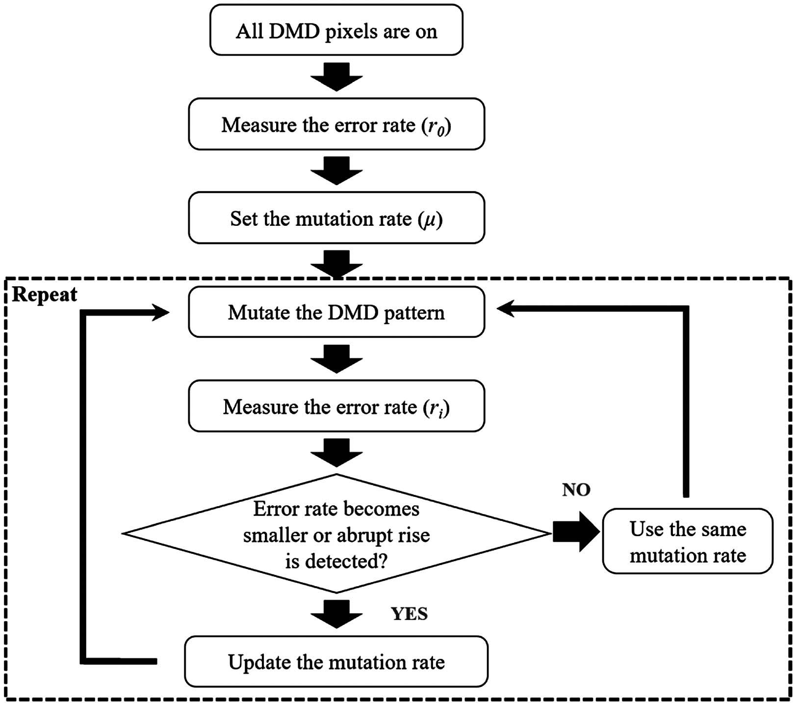
C. DMA Workflow
Figure 1.Block diagram showing the workflow of the dynamic mutation algorithm (DMA).
Figure 2.(a) Experimental setup. , ; and , ; , ; DMD, digital micromirror device; OBJ, objective lens (NA = 0.65); MMF, 1 m multimode bare optical fiber (diameter 200 μm, NA 0.22). A fiber rotator was added in the fiber rotation experiment. C1 and C2 are the fiber collimators. (b) Speckle field before optimization. (c) Focus formed after optimization by the DMA (PBR 120). The yellow lines indicate the profiles of the focus along the horizontal and vertical directions.
In the following sections, the parameters of the investigated algorithms used for the simulation and experiment are set to be the same as follows. For the DMA, the mutation constant in Eq. (13) is set to 200. For the GA, the population size is 20 and the offspring size is 10. The initial mutation rate is 0.1, which decays exponentially to a final value at 0.001. For the CSA, there is no preset parameter, whose input modes are optimized one by one with a linear rastering manner [26,27]. These initial parameters related to specific algorithms are summarized in Table 1. All these algorithms are implemented for 10,000 measurements, and each measurement is set to spend 0.2 s.
Initial Parameters Set for the DMA, GA, and CSA
Algorithm
Initial Parameter
DMA
Mutation constant 200
GA
1. Population size 202. Offspring size 103. Initial mutation rate 0.14. Final mutation rate 0.0015. Decay constant 200
CSA
None
As an example, speckle before and after DMA optimization is shown in Fig. 2. Figure 2(b) shows the speckle field before optimization, where the PBR at the target position (central point) is around 3. After wavefront shaping optimization guided by the DMA, the focus has a PBR enhanced to 120 as shown in Fig. 2(c). The full width at half-maximum (FWHM) of the focus is 15.2 and 14.5 μm in the horizontal and vertical directions, respectively.
E. Verification of the Square Rule
Figure 3.Relative PBR error rate curves ( curve). The curve based on the theoretical prediction following the derived square rule is plotted in dashed lines in both (a) and (b). In (a), the blue-diamond line shows the optimization based on the TM measured at , and the instable effect is included without remeasuring the TM for other error rates; the red-diamond line is based on the simulation with a TM, whose real part distribution is subjected to a shift (the mean of the Gaussian distribution is shifted from 0 to 0.002 in the inset). In (b), the optimal mask for each investigated error rate is reobtained to eliminate the instable effect in experiments (blue-diamond line) and simulations (red-diamond line), matching well with the theoretical curve. Relative PBR for each error rate was repeated for five executions, and the error bars show the standard deviation of the measurements.
Nevertheless, the instable medium (on the noise level) can still be governed by the square rule to some extent, but it fails to maintain accuracy. That is because the square rule is based on an unchanged and stable medium. Therefore, to experimentally recreate the square rule, at least, the time span between the generation of the optimal mask and mutated mask is limited within the decorrelation window of the medium. For example, an optimal mask is generated for every error rate investigation during the experiment. By doing so, the instable effect due to the practical medium can be almost eliminated, as shown in Fig. 3(b), where the curve attained from experiments matches well with the theoretical curve as well as the ideal simulation curve. Therefore, the square rule functions well in a real-time representation, and in other words, the error rate can provide an effective instant metric to evaluate the distance to the ideal optimal optimization. That will provide a plain yet universal perspective to analyze the imperfect focusing performance for the scattering medium, even if it is heavily perturbed.
3. RESULTS
A. Simulation
Simulations are done to evaluate the performance of the DMA, which is compared with two representative existing algorithms, i.e., the GA and the CSA. In addition to their popularity, the GA and CSA are selected because they share some similarities with the DMA. Both the DMA and GA have a mutation process and target optimization in instable environments. Meanwhile, the DMA and CSA are straightforward algorithms that do not rely much on previous results. Simulations with the DMA, GA, and CSA have been performed under various conditions of different levels of noise, and the results are compared based on the PBR throughout a fixed number of measurements (or iterations). Whenever the intensity of the target mode is measured, it is counted as one measurement, and the GA usually needs several measurements for one iteration. Each curve in the plots is an averaged result of 50 executions with a new transmission matrix generated to simulate the scattering process for every execution. input modes (modulating elements for binary-amplitude modulation) are used, and the output mode at the center is chosen for optimization.
1. Influence of Noise Level
In this section, the algorithms are compared under different levels of noise. Additive white Gaussian noise is added in every intensity measurement to mimic the instability of the optical system in the actual environment [28]. The Gaussian noises, with standard deviations of 30% and 60% of the initial average intensity , are set to represent the low-noise and high-noise situations, respectively.
Figure 4.Simulation results of the DMA, GA, and CSA under different conditions: (a) noise-free; (b) low-noise: ; (c) high-noise: ; (c)–(f) 25% right shift of the transmission matrix (at the 5000th measurement) applied to noise-free, low-noise, and high-noise conditions.
Apart from the noise caused by the instability of the optical system, optimization results can be greatly affected by the instability or slight movement of the scattering medium. To simulate this situation, a 25% right shift of the scattering medium was implemented at the 5000th measurement. The scattering medium was represented by an transmission matrix. new elements, following the same circular Gaussian distribution, are generated and inserted to the left of the matrix. The right 25% of the original matrix elements are removed so that a new transmission matrix to mimic the shift of the medium is formed. Different from the noise addition process, which only affects the intensity measurement, the shift also leads to changes in the transmission matrix. Simulations are done in noise-free, low-noise, and high-noise situations. The simulation parameters used for the algorithms here are the same as those mentioned in Section 3.A.1. Figures 4(d)–4(f) show how the DMA, GA, and CSA respond to the shift in the transmission matrix.
As seen, right after the transmission matrix is changed, there is a sudden drop of PBR in all three algorithms. The GA fails to adapt to the sudden change of the TM shift for all three investigated noise conditions, which is associated with the mechanism of the GA: the offspring (amplitude masks) with lower cost (intensity) in the population is replaced, and the best offspring is always kept [28]. Also, the whole population is generated based on the medium status before the TM shift, whose dependency and correlation regarding the largely shifted TM are relatively low. Therefore, when it encounters a relatively large enhancement drop, it is hard to produce offspring with cost (i.e., the PBR) larger than the former best one, which makes the optimization trapped in a local maximum. In contrast, the DMA and CSA successfully recover the focus after the TM shift under the noise-free and low-noise conditions. Such achievement is probably due to their absence of a pool with a large population, whose information is strongly related to the status of the medium before the TM shift. Or equivalently, the population size of the DMA and CSA is 1, so the modulating mask can be instantly guided by the information from the sudden shift without constraints from the other masks in the pool. Under the high-noise condition, the DMA is the only algorithm that can adapt to the sudden change and bounce back to the original level after measurements. The CSA, limited by its weak noise-resisting ability, fails to tackle the high-noise conditions.
As a comparison, the square rule, providing the DMD error rate from the instant PBR, shows its advances to deal with different levels of noise conditions and sudden changes. In the next section, experimental performance will be further discussed.
B. Experiment
1. Focusing Against Strong Noise
Figure 5.Experimental results of the DMA (red solid curve), GA (black dashed curve), and CSA (green dotted curve) focusing performance against strong noise.
With more apparent perturbations, e.g., a slight movement, a bending, or a small rotation to the MMF, the corresponding TM can be significantly changed and the speckle patterns decorrelated. If that occurs during the experiment, the optimization process is disrupted, and the resultant focal spot may be ruined. In this section, experiments were done to study how perturbations, with rotation to the MMF as an example, affect the optimization, and how different algorithms respond to such heavy instability. The same experimental setup was used with an additional fiber rotator, which can rotate the MMF with various angles.
Figure 6.(a) Relationship between fiber rotation and PBR drop. (b) Measurement required to rebound for different degrees of fiber rotation. Each dot in (a) and (b) is averaged from five executions, and the error bars show the standard deviation of the measurements. The optimizations in (a) and (b) are realized by the DMA. (c) Experimental focusing performance of the DMA in response to 2.5°, 5°, and 7.5° fiber rotation.
Figure 8.Focal spots at four different stages with different algorithms: before optimization (zeroth measurement), before fiber rotation (5000th measurement), right after 5° fiber rotation (5001st measurement), and after reoptimization (15,000th measurement). The 150 μm scale bar is applicable to all images in this figure.
The recovery efficiency of the CSA may depend on when the perturbation occurs. In the experiment, as the perturbation is induced when the optimizing elements are near the edges of the DMD, the recovery speed is slow. More importantly, merely changing one element for each measurement in the CSA is not efficient to overcome the instability since the positive contribution from one element is probably below the noise level. In contrast, the GA cannot obtain further PBR after the rotation, as the optimization is trapped in the local maximum due to three reasons. First, the optimizing masks in the population library are merely based on the medium status before perturbations. Second, the decorrelation due to 5° rotation cannot be tolerated or generalized from that of the population generated via GA. Third, the mutation process in the GA is not adaptive to the sudden perturbations during optimization since the mutation rate in the GA is exponentially decayed regardless of the focus degrading. Collectively, the DMA can effectively battle those defects inherently embedded in the CSA and GA, which are also shared by most of the popular algorithms.
4. DISCUSSION
As seen, the simulation and experiment results have demonstrated the high adaptability of the DMA. It performs comparably with the GA in a noisy environment and overcomes the heavy perturbations with a robust recovery ability. Apart from this distinctive adaptability, the ease of implementation is another advantage of the DMA. For the GA, several key parameters, such as population size, offspring size, and mutation rates, need to be adjusted appropriately at the beginning [28]. However, in DMA, only one parameter is required to be set, which is the mutation constant, a number bounding the mutation rate. Benefitting from the error rate and the square rule, the optimization error in the modulating mask can be easily quantified, causing the whole optimization process to be straightforward. It is simply based on real-time measurements, and it is less likely to be affected by the improper selection of parameters. Also, the error-rate-based DMA does not strongly depend on the modulating mask in previous iterations, and therefore adaptability can be effectively achieved to deal with dynamic media. As an example of the square rule’s applications, the DMA does show its capability to adapt to strong and/or sudden perturbations benefitting from the use of the practical metric, the error rate. Note that the metric can also be incorporated into other optimization methods, such as the GA, to improve adaptability.
Although only one of the numerical optimization methods, i.e., the GA, is chosen for demonstration in this study, others, such as the SA and PSO, are similar. Including in their pools a large population of masks, the mechanisms to generate new modulating patterns originate from the philosophy of numerical optimization: (1) the portion of the modulating elements to be mutated is preset or decays with certain rules; (2) the monitored PBR is used to produce an acceptance probability of the newly generated masks or to update the mask. These two mechanisms ensure the generalization to the noise, even on the scale of [33], around a specific equilibrium of the medium. However, a sudden strong perturbation behaves differently since the equilibrium of the medium has been considerably changed, and the experience based on the previous equilibrium is “out-of-date” as discussed in the last section. Therefore, it can be considered that the physics-based square rule probably enhances the adaptability of the existing methods. Notably, if a new parameter is incorporated in those methods, other parameters probably need to be further tuned to match the function of the square rule, which is a nontrivial manipulation. Incorporation of other optimization algorithms with the square rule is therefore beyond the scope of this paper.
5. CONCLUSION
In this study, a simple square rule of binary-amplitude-modulation-based wavefront shaping optical focusing based on universal strong scattering media has been theoretically obtained. With this rule, the real-time error in the modulating mask can be simply calculated from the concurrently measured PBR of the optical focus. Based on such a real-time metric, a novel feedback-based wavefront shaping algorithm, the DMA, has been proposed. Both the simulation and experimental results have demonstrated its high adaptability and unique recovery ability that no other existing algorithms can achieve: focusing of diffused light can be regained without re-running the optimization even after a 60% drop of the PBR. This is due to the application of the square rule, which guides the optimization with universal physics knowledge about the strong scattering process instead of a random guess. Notably, the square rule assumes that the transmission matrix of a medium follows a circular Gaussian distribution. It can be easily fulfilled when the transmitted medium is a strong scattering medium: photons are multiply scattered, and most of these scattering events are independent [39]. Therefore, the square rule between the DMD error rate and the degraded focus can be generally applied to the process in a strong scattering regime. The algorithm is therefore particularly suitable to be used in heavily instable or motional scattering environments. Note that the DMA in this study merely serves as an example application to utilize the error rate and square rule to optimize the single-point focusing. On the other hand, MMF is used as the example of scattering media in this study, so that by applying rotation of certain degrees we can induce controllable, repeatable, and quantifiable perturbations to the resultant speckle patterns. This is necessary for the current phase of the proof of principle, although it is not ideal. With further improvement, we believe the study may boost or inspire many applications of wavefront shaping with instable media or even living biological tissue.