C. J. Zhu1、2、3, K. Hou1、4, Y. P. Yang1、6、*, and L. Deng5、7、*
Author Affiliations
1MOE Key Laboratory of Advanced Micro-Structured Materials, School of Physics Science and Engineering, Tongji University, Shanghai 200092, China2School of Physical Science and Technology, Soochow University, Suzhou 215006, China3Collaborative Innovation Center of Light Manipulations and Applications, Shandong Normal University, Jinan 250358, China4Department of Mathematics and Physics, Anhui Jianzhu University, Hefei 230601, China5Center for Optics Research and Engineering (CORE), Shandong University, Qingdao 266237, China6e-mail: yang_yaping@tongji.edu.cn7e-mail: lu.deng@email.sdu.edu.cnshow less
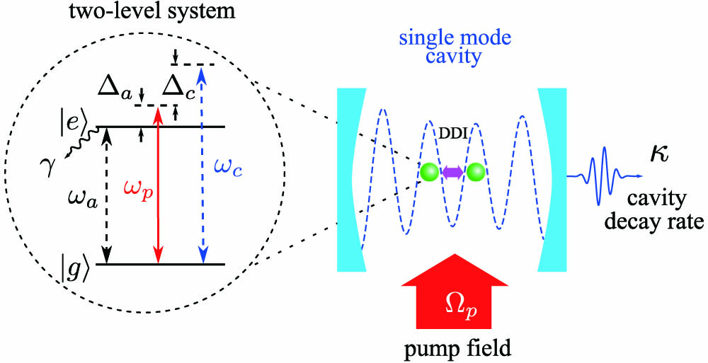
Fig. 1. Sketch of the two-qubit cavity QED system with different cavity mode frequency ωc and qubit resonant frequency ωa. A pump field Ωp couples the qubit ground state |g⟩ and excited state |e⟩ with the angular frequency ωp. γ and κ denote the qubit decay rate and the cavity decay rate, respectively. Here, DDI represents the dipole–dipole interaction when two qubits are close enough.
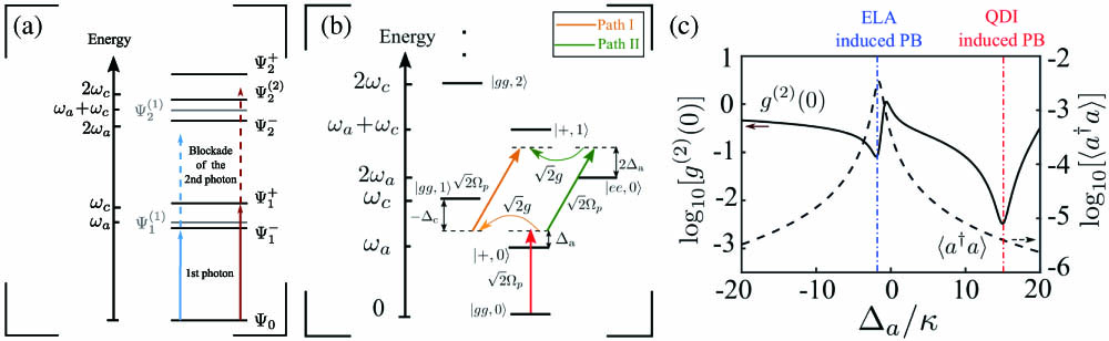
Fig. 2. (a), (b) The anharmonic ladder-type energy structure and the destructive interference pathways for the ELA-based and QDI-induced PBs, respectively. In (a), the absorption of a second photon of the pump field will be blocked due to the large energy mismatch if the pump field is tuned to the state Ψ1(±) as denoted by the blue and red arrows, respectively. In (b), two interference pathways from state |+,0⟩ to state |+,1⟩ are indicated by the yellow and green arrows, respectively. (c) The equal-time second-order correlation function g(2)(0) (solid curve) and mean photon number ⟨a†a⟩ (dashed curve) as a function of the normalized detuning Δa/κ. Here, we chose J=0, Δc=−30κ, g=5κ, γ=κ, and Ωp=0.1κ.
Fig. 3. Logarithmic plots of (a) the second-order correlation function g(2)(0) and (b) the mean photon number ⟨a†a⟩ as functions of the normalized detuning Δa/κ with the DDI strength J=0 (black curves), g (blue curves), and 3.5g (red curves), respectively. The green dashed line indicates the condition Δc=−2Δa. Other system parameters are the same as those used in Fig. 2(c).
Fig. 4. Logarithmic plots of (a) the second-order correlation function g(2)(0) and (b) the mean photon number ⟨a†a⟩ as functions of the DDI strength J/g and detuning Δa/κ by setting Δc=−2Δa and g=5κ. Other system parameters are the same as those used in Fig. 3. The dashed curves denote the optimal condition g2=−Δa(Δa−J).
Fig. 5. Logarithmic plots of (a) the second-order correlation function g(2)(0) and (b) the mean photon number ⟨a†a⟩ against the detuning Δa/κ and coupling strength g/κ with Δc=−2Δa and J=2g. The white dashed line corresponds to the condition g=Δa, while the black solid curves denote g(2)(0)=0.01.
Fig. 6. (a) The second-order correlation function log10[g(2)(0)] versus the normalized pump field Rabi frequency Ωp/κ with spontaneous decay rate γ/2π=0.1κ (red solid curves), 0.5κ (black dashed curves), and κ (blue dotted curves), respectively. (b) The plot of the photon number in Fock states with Ωp=0.2κ. Here, the system parameters are given by g=2κ, and J=Δc=−2Δa=2g.
Fig. 7. Logarithmic plot of (a) the equal-time second-order correlation function g(2)(0) and (b) the mean photon number ⟨a†a⟩ as functions of the normalized atomic detuning Δc/κ and the cavity detuning Δa/κ. The white dashed–dotted curves denote the condition of the ELA-based PB [i.e., Eq. (6)], and the white dashed lines denote the condition of the QDI-induced PB [i.e., Eq. (10)]. The system parameters are given by Ωp=0.1κ, g=5κ, and γ=κ.
Fig. 8. Logarithmic plot of (a) the equal-time second-order correlation function g(2)(0) and (b) the mean photon number ⟨a†a⟩ as functions of Δc/κ and Δa/κ with J=2g. The white dashed–dotted curves denote the condition of the ELA-based PB [i.e., Eq. (13)], and the white dashed lines denote the condition of the QDI-induced PB [i.e., Δc=−2Δa].